Regularized likelihood methods

• Regularized likelihood methods
  • Regulaization
  • Ridge - L2 regularization
  • Lasso - L1 regularization
  • Beyond Lasso
  • Summary

Regularized likelihood methods

Regulaization

Regularization is the approach for regression model with regularized likelihood methods. And it also used to understand the sparse modeling.

Regression is a statistical processes for estimating the relationship among variables, and usually have this form,

$$y = f(x; \Theta) = x_1 \theta_1 + x_2 \theta_2 + \cdots + x_d \theta_d + \epsilon$$

Seen above, the model can be expressed with independent variable $x$ and dependent variable $y$, the weight parameter $\Theta$ and noise $\epsilon$.

In general, the goal of regression is to find an approximated function using weight parameter $\Theta$ for each dataset points. To find the optimal weight parameter, we usually select $\Theta$ with minimum error (cost, loss, whatever) between the prediction and actual datapoint. In this case, simplest way is to take the sqaured mean error, and get the argument when the error is occurred, this is called Ordinary Least Square (OLS for short)

$$\hat{\theta}_{\text{LS}} = \arg\min_{\theta} \sum_{i=1}^n (y_i - f(x_i;\theta))^2$$

With this error, the overall solution minimizes the sum of the squares of residuals.(also known as R-squared).

Another candidate for error function is Maximum Likelihood,

$$\hat{\theta}_{\text{ML}} = \arg\max_{\theta} \sum_{i=1}^n \log (y_i \vert x_i ; \theta )$$

The formulation seems difficult, but it means that find the weight that generates maximum log probabilty of $y$ given $x$. In general, OLS and Maximum Likelihood derives the same solution when the noise $\epsilon$ follows the normal distribution with zero mean ($\epsilon \sim N(0, \sigma^2)$)

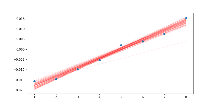
Back to the previous linear regression example. There is no perfect model for fit. Instead, we can approximate model with form of independent variables. We can make multiple models, from simple model to complex model, which is $d$th degree polynomial.

$$\begin{aligned} f_2(x;\theta) &= x_1 \theta_1 + x_2 \theta_2 + \epsilon \\ f_3(x;\theta) &= x_1 \theta_1 + x_2 \theta_2 + x_3 \theta_3 + \epsilon \\ f_d(x;\theta) &= x_1 \theta_1 + x_2 \theta_2 + \dots + x_d \theta_d + \epsilon \end{aligned}$$

More complicated model will be accurated for given dataset, but it will lose the generalization. There is a tendency that the more parameters we use, it is more likely that model would be overfit. Of course, simplest model occurs underfitting problem.

So to prevent the overfitting problem, we can apply regularization term for penalizing complicated model. And it can expressed the symbol $\Psi$. If we use cost fuction for finding the optimal weight $\theta$, we can express like this,

$$\hat{\theta} = \arg \min_{\theta} ( \mathcal{L(y, f(X; \theta)) + \lambda \Psi(\theta)})$$

Ridge - L2 regularization

Rigde Regression (Hoerl & Kennard, 1970), also known as L2 regularization, is used L2 norm as a penalty term and regularization.

$$\hat{\theta} = \arg \min_{\theta} (\Vert y - f(X;\theta) \vert_2^2 + \lambda \Vert \theta \Vert_2^2)$$

In this case, a larger weight parameter in squared scale can be said to be more complex than a lower weight parameter. Using this, we can quantify the complexity of the model.

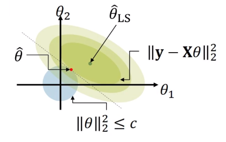
If we define some constant $c$, and limitation for regularization subject to $\Vert \theta \Vert_2^2$, we can find the parameters that minimize the residuals within that complexity, which is least squares. Here in figure, the upper bound of complexity constraint $c$ is expressed as blue region. In this case, least square has a minimum value on a contact point with blue region, and this point might be the parameter is L2 regularization. And it is said that the ridge regression shrinks $\theta_j$ to non-zero.

Since the L2 regularization term contains the quadratic form, it is strictly convect, continuous, and differentiable with respect to $\theta$. So we can get closed form solution, and get an argument of minima by taking a derivative with respect to $\theta$ and equate to 0.

So how can we get closed-form solution? If we set $\lambda=0$, we can get least squared term. So we can differentiate it,

$$\hat{\theta} = \hat{\theta}_{\text{LS}} = \arg \min_{\theta}(\Vert y - X\theta \Vert_2^2) = \arg \min_{\theta}((y-X\theta)^T (y - X\theta))\\ \frac{\partial (y-X\theta)^T (y - X\theta)) }{\partial \theta} = \frac{\partial [y^Ty - y^T X\theta - \theta^T X^T y + \theta^T X^T X \theta]}{\partial \theta} \vert_{\theta = \hat{\theta}_{\text{LS}}} = 0$$

At this case, we can make numerator to 0 for minimizing.

$$y^Ty - y^TX\theta - \theta^T X^T y + X\theta^T X\theta = 0 \\ \hat{\theta}_{\text{LS}} = (X^TX)^{-1}X^Ty$$

What if $\lambda > 0$, then the regularization term is remained and we can differentiate this form.

$$\hat{\theta}^{*} = \arg \min_{\theta}(\Vert y - X\theta \Vert_2^2) = \arg \min_{\theta}((y-X\theta)^T (y - X\theta) + \lambda \theta^T \theta) \\ \frac{\partial (y-X\theta)^T (y - X\theta) + \lambda \theta^T \theta) }{\partial \theta} = \frac{\partial [y^Ty - y^T X\theta - \theta^T X^T y + \theta^T X^T X \theta + \lambda \theta^T \theta]}{\partial \theta} \vert_{\theta = \hat{\theta}^{*}} = 0$$

In this case,

$$-X^Ty = X^Ty + (X^TX+ X^T X) \hat{\theta}^{*} + 2 \lambda \hat{\theta}^{*} = 0 \\ \hat{\theta}^{*} = (X^TX + \lambda I)^{-1}X^Ty$$

So we can summarize its soluntion in terms of $\lambda$

• $\lambda = 0 \rightarrow \hat{\theta}_{\text{LS}} = (X^TX)^{-1}X^Ty$
• $\lambda > 0 \rightarrow \hat{\theta}^{*} = (X^T X \lambda I)^{-1} X^Ty$

In case of $X_i$ are independent and identically distributed(so called i.i.d) with standard normal distribution,

$$X^TX = I \text{ and } \hat{\theta}^* = \frac{1}{(1 + \lambda)} \hat{\theta}_{\text{LS}}$$

Through this, we can imply that when the regularization parameter is used, weight parameter shrinks in propotional to the regularization parameter.

Lasso - L1 regularization

Unlike ridge regression, Lasso used L1 norm for regularization term. L1 norm is absolute value of magnitude.

$$\hat{\theta} = \arg \min_{\theta}(\Vert y - X\theta) \Vert_2^2 + \lambda \Vert \theta \Vert_1)$$

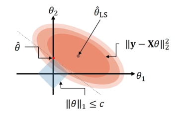
The difference between ridge and lasso is the range of constraint $c$.

so we can also expressed like this,

$$\hat{\theta} = \arg \min_{\theta} \Vert y - X\theta \Vert_2^2 \text{ subject to } \Vert \theta \Vert_1 \leq c \text{ for some } c > 0$$

The key difference between ridge and lasso is that lasso regression $\theta_j$ to 0 but also foce some of $\theta_j$ to be exactly 0. That remove some unimportant features, which became exactly zero that can be understood as sparse modeling.

Beyond Lasso

But Lasso regression has some limitations. Lasso tends to select at most n variables before it saturates. Shortly speaking, there are few data points and many features. Usually, more dataset is efficient than having many feature variables. But lasso suffered from this after saturation. This problem is called “Large p, small n”, and also known as Curse of dimensionality.

And another limitation is to ignore the correlation among grouped variables. So it might occur the information loss.

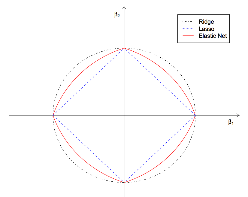
So to overcome the limitation, Elastic Net ( Regularization and Variable Selection via the Elastic Net ) is introduced. Elastic Net regression combines the lasso and ridge regression as an regularization term.s

¹

and form is like this,

$$\arg \min_{\theta} ( \Vert y - X\theta \Vert_2^2 + \lambda_1 \Vert \theta \Vert_1^2 + \lambda_2 \Vert \theta \Vert_2^2)$$

In this model, L1 norm (the Lasso regularizer) generates the sparse modelm L2 norm (the ridge regularizer) removes the limitation on the number of selected variables, and it stabilizes the selection from grouped variable, which was the problem while using only Lasso regression.

In summary, the Elastic net performs variable selection and continuous shrinkages to select groups of correlated variables at the same time. Usually, we use cross validation of different combination of $\lambda_1$ and $\lambda_2$ to find the best values.

And another approach is Group Lasso ( Model selection and estimation in regression with grouped variables ) Suppose that we have huge amounts of data with gropu features appear sequentially. Maybe we want to find the important variables on the group level, not independently. Usually, this kind of high dimensional data have structured into $q$ groups, and have total $j$ variables.

$$g_1, \dots, g_q \subseteq \{1, \dots, J\}, \text{ disjoint and } \bigcup_g G_g = \{1, \dots, J\}$$

Mentioned in previously, if we use Lasso for selecting variables, lasso selects the variables regardless of group correlation.

But Group Lasso can consider the group property, so all the member of a particular group are either included or not included.

Because the penalty is reduced to the L2 norm on the subspeces defined by each group, it is not possible to select only some correlated variables of a group as a ridge regression can not.

$$\arg \min_{\theta} \Big(\sum_{j=1}^J(y_j - \theta_j x_j)^2 + \lambda \sum_{j=1}^J \sqrt{p_j} \Vert \theta_j \Vert_2^2 \Big)$$

Note that, $\sqrt{p_j}$ is the varying group sizes acting as a penalty matrix. And $\theta_j$ is the coefficient vector of group $j$. Here, the penalty is the sum of difference of space norms as in the standard Lasso, it may contain some non-differentiable points in the constraint that corresponds to some subspaces being equally zero. Therefore, we can set the coefficient vector for sums of spaces to zero, while only shrinking others.

Summary

We covered the regularized likelihood methods for regression, the Ridge Regression and the Lasso Regression. And there are some limitation for selection variable in specific conditions. To overcome this, Elastic Net (combining Ridge and Lasso) and Group Lasso is introduced.

1. Figure from jamis.eth ↩