Perceptron and its convergence theorem
Perceptron algorithm is used for supervised learning of binary classification. In this post, it will cover the basic concept of hyperplane and the principle of perceptron based on the hyperplane. And explains the convergence theorem of perceptron and its proof. This post is the summary of "Mathematical principles in Machine Learning"
Perceptron and convergence theorem
Motivation

There are lion and tiger. How can we discriminate Lion and Tiger? Someone said that:
- Tiger has stripe on its head
- Lion has mane on its head
This information such as striped pattern and the mane is called features in the machine learning.
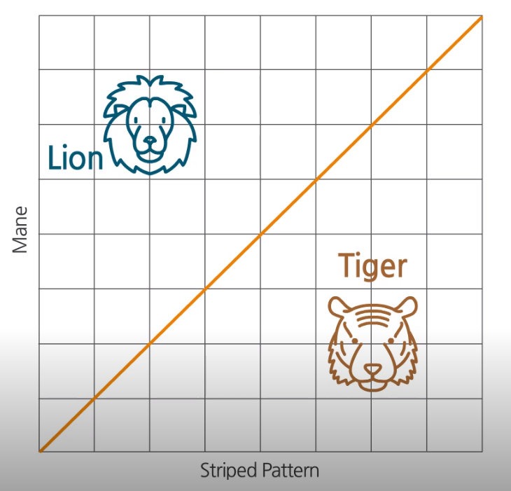
How can we make Intelligence to classify Lion and Tiger automatically? If we can map each creature into feature space, we can divide them with a line and classify as lion for the data above the line, and classify as tiger for the data below the line. At this case, the line regards as an intelligence distinguishing lion and tiger.
To generalize this problem, we have 2 types of label (Class1 and Class2). And each data has 2-dimension coordinates.
Then, we can define the line $f(x) = x_2 - x_1$. If $f(x) > 0$, it must be Class1, and if $f(x) < 0$, then it must be Class2. Our goal is to introduce the algorithm for finding the function from the data.
Hyperplane
The line in the previous example is called as a hyperplane in a high dimensional space. The hyperplane can be defined in the arbitrary D-dimensional space and should separate the defined space into two disjoint spaces.
In mathematical form, it relates to normal vector $W$ and bias $b$. Especially, the hyperplane can be represented by the inner product between the normal vector and the data points in the input space, then adding bias.
For example, consider a 2-dimension example.
In this case, hyperplane $f(X)$ is:
And we can call $W$ as normal vector of the hyperplane (unnormalized)
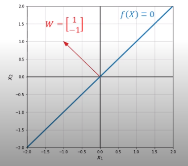
The red line is normal vector, and blue line is hyperplane. As you can see this, the normal vector is orthogonal ($90^\circ$) to any vector or data point lying on the hyperplane. As a result, hyperplane is defined by an normal vector and bias.
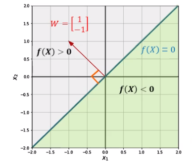
We can color the region based on the sign of the output of the hyperplane. In the previous example, the hyperplane itself has 0. So it is also called decision boundary
Perceptron
So we found out that to handle binary classification, we need to find hyperplane from the given data. How can we do that?
One answer is Perceptron. Perceptron is an algorithm for supervised learning of binary classification problem. It requires the training dataset that includes Input $X$ and Corresponding label $y$.
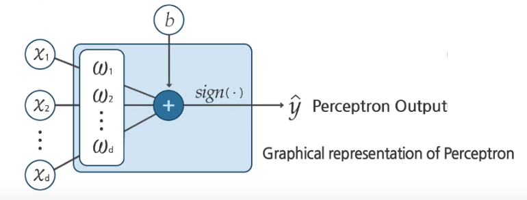
From the figure, we can guess the prediction process of the perceptron briefly. The sign of sum of all value becomes the predicted label. In details, the sum of value is decomposed by inner product between the weight of the perceptron and the input vector, and adding bias.
This process is similar with the definition of the hyperplane. So we can use this algorithm to find the hyperplane.
For example,
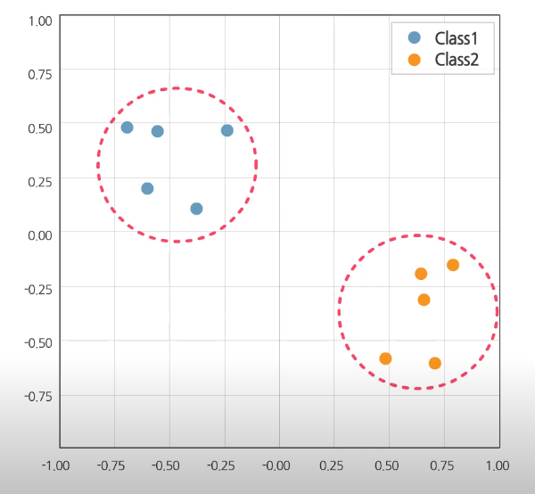
Given training dataset,
Class 1 has label 1 and Class 2 has label -1. For ease of expression, we uses homogeneous coordinate representation in $X$
From this, we can define the hyperplane.
To use perceptron,
- Initialize the normal vector and bias
- For $t = 1 \dots T$ (The number of iteration)
Note: $\text{sign}(x) = \begin{cases} -1 & \quad x > 0 \ 0 & \quad x = 0 \ 1 & \quad x > 0 \end{cases}$
- $f(X_n) = \text{sign}(W^T X_n)$
- If $y_n \neq f(X_n)$, then update $W = W + y_n x_n$ else, leave $W$ unchanged.
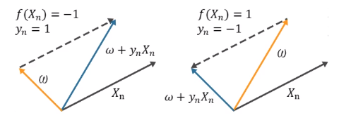
Convergence for the perceptron
Anyway, The question remains that “Does the perceptron algorithm will converge or not?” And, the answer is YES. If the data is linearly separable, its algorithm converges.
There are theorems related on the convergence for the perceptron:
- Number of update $k$ is bounded in the perceptron algorithm with 2 assumptions.
- Assume that there exists some weight vector $W^$ such that $\Vert W^ \Vert = 1$, and some $\gamma > 0$ such that for all $n = 1 \dots N$
Where $\Vert \chi \Vert$ is 2-norm of $x$ (i.e. $\Vert x \Vert = \sqrt{\sum_i x_i^2}$)
- Assume in addition that for all $n$,
From these assumption, the perceptron algorithm have the number of update $K$ is bounded.
- At first, define $W_k$ to be the weight bector when the algorithm makes its $K$th update.
- Suppose the weight vector is initialized zero vector at the first state ($W_1 = 0$)
- Next, assuming the weight vector at $K$th update on example $n$, we have,
- It follows by induction on $K$ (recall that $\Vert W_1 \Vert = 0$)
-
In addition, because $\Vert W_{k+1} \Vert \dot \Vert W^* \Vert \geq W_{k+1}^T W^*$ (from definition of inner product) and $\Vert W_1 \Vert = 0$, we have $\Vert W_{k+1} \geq k \gamma \Vert$ (This is the lower bound of $\Vert W_{k+1} \Vert$)
-
In the second part of the proof, we will derive an upper bound of $\Vert W_{k+1} \Vert$
- It follows by induction of $k$ (recall that $\Vert W_1 \Vert^2 = 0$)
And this is the upper bound of $\Vert W_{k+1} \Vert^2$
Combining the lower bound and upper bound
Then, we can get the upper bound for the number of update $k$
As you can see, the boundary is existed in some range. So we can find out that perceptron algorithm has finite update in the training process.
One hyperplane separates the space into 2 half-space. But if the data is not linearly separable, althought the task is binary classification, one hyperplane cannot discriminate labels. In this case, more perceptrons are required to get better result. More effective way to handle is to add the depth(meaning a set of perceptrons) with non-linear function (also known as activation function) We call it Multi Layer Perceptron (MLP) or neural network. If you want the visualization of neural network, check out the following links:
Summary
In this post, it introduced the perceptron algorithm which trains the hyperplane, and tried to look the update rule in the perceptron. Also, we prove the theorem related to convergence for the perceptron.