Convexity of Linear Hypothesis and Margin Bound of Linear Classifiers

• Convexity of Linear Hypothesis and Margin Bound of Linear Classifiers
  • Theoretical Analysis on Classifications with Linear Hyperplanes
  • VC-dimension generalization bound
  • Summary

Convexity of Linear Hypothesis and Margin Bound of Linear Classifiers

Theoretical Analysis on Classifications with Linear Hyperplanes

At first, assume that we have a shattered set. If we have a set $A$ and $C$ is a class of sets, the class $C$ fully shatters the set $A$ if for each subset $a$ of $A$, there is some element $c$ of $C$ such that:

$$a = c \cap A$$

For example, consider the set of two points on the line. Points in the interval will get the “+” label.

In this case of two points, Class of set $C$ has four intervals (“–”, “+-“, “++”, “-+”), and the set of two points is set $A$ (“+-“, “-+”)

Expand it with three point. Consider the set of three points, one set of three points has “+-+”

In this case, it cannot separate the set with intervals. How can we explain it with mathematical definition?

New concepts called VC-dimension is derived. The VC-dimension of a hypothesis set is defined by:

$$VC(H) = \max \Big\{m: \prod_h (m) = 2^m\Big\}$$

VC-dimension is the expression of maximum intervals for separating sets. And it is the size of the largest set that can be fully shattered by $H$.

Back to the previous example, as you can see, we cannot separate the interval with three points, just two points can go on. Thus,

$$VC(\text{intervals in }\mathbb{R}) = 2$$

That is, 2 real numbers are fully shattered by the set of intervals.

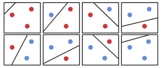
In the example figure, any three non-colinear(meaning that no points are in the same line) can be shattered in 2D. It can just separate 2 and 1 or 3 and 0, and it cannot separate the point individually. Thus,

$$VC(\text{hyperplanes in }\mathbb{R}^2) = 3$$

As you can see from another example, if we consider to separate $d+1$ points, it requires the hyperplane in $R^d$. Thus,

$$VC(\text{hyperplanes in } \mathbb{R}^d) = d + 1$$

VC-dimension can be applied in arbitrary hypothesis, but in this post, it just focus on the linear hypothesis case. The Linear hypothesis set is the set that parameterized by a linear vector $\mathrm{w}$ such that,

$$h_{\mathrm{w}} (x) = <\mathrm{w}, x> = \mathrm{w}^T x$$

This form is similar with the expression of hyperplane in previous post. So it can be represented by a hyperplane.

VC-dimension generalization bound

In the machine learning task, we want to predict something or gather some information for future. To do this, we usually wish to bound the generalization error ($R(h)$) in some hypothesis ($h$) given the empirical error ($\hat{R}(h)$) computed with $m$ samples.

In this case, Generalization error is measured with the original distribution, and it will give us a generalized performance of trained model.

We can derived the generalization bound with a sort of inequality (also known as VC-inequality) form:

$$\mathcal{R}(h) \leq \hat{\mathcal{R}}(h) + \sqrt{\frac{2 (N+1) \log \frac{em}{N + 1}}{m}} + \sqrt{\frac{\log \frac{1}{\delta}}{2m}}$$

Note: this inequality is under the condition with hypothesis $h$ and high probability (at least $1 - \delta$)

Note: The number $N+1$ expressed in second term comes from the definition of VC-dimension. Because VC-dimension of hyperplanes in $N$ dimensional space is $N+1$

In the form, Generalization error is bounded by the sum of empirical error ($\hat{\mathcal{R}}(h)$) and function of VC-dimension (second term) and number of samples ($m$)

But if $N \gg m$ (meaning that the dimensional space is higher than the number of samples), second term in the square root will be negative, thus we cannot find the solution in $\mathbb{R}$, and the bound is uninformative. But some approaches like Support Vector Machine can handle this in high dimensional space.

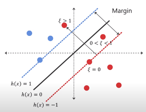
Anyway, to explain the linear model in high dimensional space, it is required another kind of generalization bound. In this case, margin of the hyperplane will be considered.

Let assume that there are sample inside the circle which radius is $r$,

$$S \subseteq \{ x: \Vert x \Vert \leq r \}$$

In this case, the VC-dimension of hyperplane can be expressed like this,

$$H = \{ x \rightarrow \text{sign}(\mathrm{w} \cdot x) : (\min_{x \in S} \vert \mathrm{w} \cdot x \vert = 1) \cap ( \Vert \mathrm{w} \Vert \leq \Lambda)\}$$

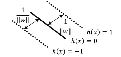
here, $\Lambda$ is related to the margin of the hyperplane.

$S$ is subset of circle which has $r$ radius. Of course, maximum value of $S$ will be on the boundary of circle. So we can derive the upper bound of VC-dimension with margin factor $\Lambda$ and radius $r$ of the sphere containing the data. (Check the details for proof here)

$$VC \leq r^2 \Lambda^2$$

In the previous example, VC inequality has a problem from the high dimensional space($N+1$). But we can substitute this to maximum boundary of sphere ($r^2 \Lambda^2$), then,

$$\mathcal{R}(h) \leq \hat{\mathcal{R}}(h) + \sqrt{\frac{2 \cdot r^2 \Lambda^2 \log \frac{em}{r^2 \Lambda^2}}{m}} + \sqrt{ \frac{ \log \frac{1}{\delta}}{2m}} \quad \text{When } m \geq VC$$

As a result, we can clearly explain the linear models with new generalization bounds. From the expression, we can get that as $\Lambda$ becomes small, the margin of the hyperplane becomes larger. And the value of bound will be tigher in the generalization bound, cause the second term of expression will be smaller.

Summary

In this post, it is introduced the theoretical analysis of classification with linear hyperplanes. There are many candidates for hyperplanes, but it requires a boundary to explain good or bad. So generalization bounds is expressed. Here, VC-dimension is mentioned, and it has a problem in high dimensional space. To handle this, margin is used to limit the upper bound. Through this, we can clearly explin the linear model with new generalization bound.