Overview of Sparse Modeling
In this post, it will be explained about what the sparse modeling is and why this algorithm is used. This post is the summary of "Mathematical principles in Machine Learning" offered from UNIST
Overview of Sparse Modeling
Sparse modeling
The definition of sparse is come from the distribution. Sparse means something that is small number or amount and spread out over an area(or distribution). For example, sparse vectors and matrix have most of zeros and only a few number of non-zero valued elements. So why do we bring the concept of sparse to Machine Learning?
Sparse modeling has advantages from training model. For example, consider about simple linear regression.
When creating a polynomial regression model(meaning that have many terms of coefficients), the model can be expressed as a vector of polynomial coefficients. If the model is overtrained, in other words, all coefficient(or weight) vector have non-zero value, model will be overfitted. On the other hands, if the coefficient vector has most of zeroes, then the regression model cannot represent the actual data (underfitted). That is, if the coefficient vector tends to be sparsed with non-zero values, the model is considered as a good fitting model. As a result, Sparsity helps to model for regularization and it prevents model from overfitting.
Another advantage from sparsity is variable selection. If we define a model as sparse, it means that some dependent variables represented by 0 are not used to predict. So we can analyze the performance of model from selected variable. That is called model interpretability.
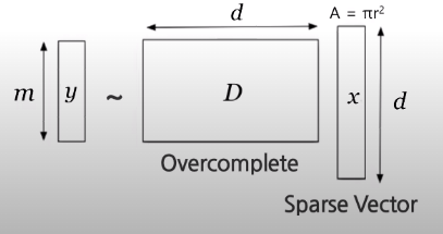
Consider about this example.

$y$ is the object we want to interpret. And $D$ is dictionary matrix to make $y$, and $x$ is sparse vector for deciding which vector is used from $D$. So our purpose is that minimizing the difference between $Y$ and the matrix multiplication of $W$ and $X$. Also for the regularization, we can add regularization term. As a result, criteria of this example can be expressed like this:
Above formula, first term is the square of L2-norm(also known as Euclidean distance),and second term is L0-norm(cardinality) of X. If the the number of zeros in the sparse vector is large, the regularization term has small value. That is, sparse vector becomes more sparse.
Let’s look at more precisely about the definition of norm. Actually, norm is the length of vector in terms of $p$. The mathematical expression of vector norm is like this:
Consider about this simple case. If we have $x=(0, -2, 0, 1, 0, 3)$, we can define the norm in terms of $p$:
| p | calculation | $\Vert x \Vert_p$ |
|---|---|---|
| 0 | $\Vert x \Vert_0 = \sharp {i \vert x_i \neq 0}$ | 3 |
| 1 | $\Vert x \Vert_1 = (\vert 0 \vert + \vert -2 \vert + \vert 0 \vert + \vert 1 \vert + \vert 0 \vert + \vert 3 \vert)$ | 6 |
| 2 | $\Vert x \Vert_2 = (\vert 0 \vert^2 + \vert -2 \vert^2 + \vert 0 \vert^2 + \vert 1 \vert^2 + \vert 0 \vert^2 + \vert 3 \vert^2)^{1/2}$ | $\sqrt{14}$ |
| $\dots$ | ||
| $\infty$ | $\Vert x \Vert_{\infty} = \max_{i=1, \dots, d} \vert x_i \vert$ | 3 |
If the vector x has a property of $\Vert x \Vert_0 \leq K$, $x$ is called $K$-sparse vector. From the example, $x$ is 3-sparse vector.
Problem of Sparse Modeling
We already expressed the criteria of specific sparse modeling, but we can generalize its form,
The first term is loss function for quantifying the goodness of approximation. So it tries to minimize the error between $Y$ and $DX$. And second term is regularization term as explained, it evaluates sparseness of coefficients(or dictionary). If this value is small, we can say that the model is more sparse and explainable.
In the next post, it will cover the mathematical approaches to handle sparse modeling, the Matrix decomposition,and also explained about backgrounds for regularization.
Summary
To avoid overfitting and regularization errors, the sparse model is represented, and it is one of the explainable artificial intelligence method. We’ll cover the various mathematical backgrounds for interpreting and extending sparse models in the next post.