Causal Bayesian Network

• Causal Bayesian Network
  • Granger Causality
  • Compare predict performance
  • Practical definition of Granger causality
  • Extensive to Multivariate Time Series
  • Summary

Causal Bayesian Network

Granger Causality

Finding a causality between these time series data is like getting knowledge from the data. For example, suppose we observed the coal consumption from decades. And it led to an increase in atmospheric carbon dioxide concentration, which affect the global temperature. In this case, temporal causality is the causal relationship between time series data.

Granger Causality is kind of temporal causality, and it describes the relationship between two time series data. Here are some basic principles.

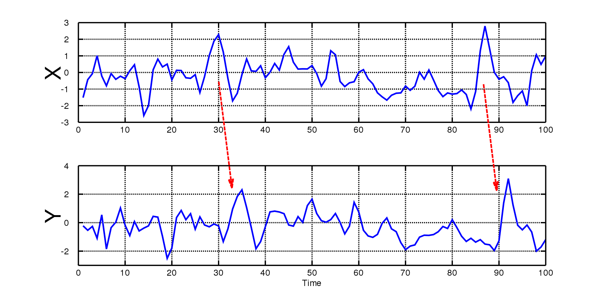
First, a cause is prior to its effect. In this picture, we can see similar patterns from two figures. After the prior event occurs in cause and after a certain time, its effect is also observed in other time series data. Then, we assume that prior event maybe affect the post event. In this case, Granger Causality is caused by temporal order of event.

We covered the definition of causality in the previous post. But Granger causality is different from them because of its temporal ordering characteristics, meaning its causal information contains temporal properties.

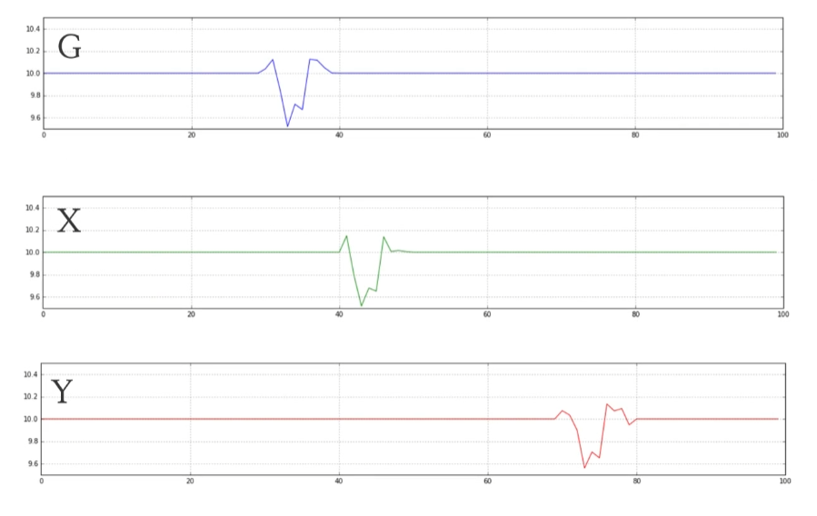
Suppose we have three event, $G, X, Y$, and $G$ affects the $X$ and $Y$. So $X$ and $Y$ has causality with $G$. And as you can see, the influence caused by $G$ appears at different times in $X$ and $Y$. From this figure, we can notice that $G$ is main cause of $X$ and $Y$.

But think about that we don’t know about $G$, only know $X$ and $Y$. We may assume that $X$ and $Y$ have sort of temporal causality between them.

As a result, we can not ignore the possibility that there might be a real cause compound, like $G$. In this case, $X$ and $Y$ are Granger Causality.

Let’s consider another example, the chicken and egg problem. Which came first, the chicken or the egg? And is there a correlation between the number of chickens and the number of eggs? If it is, did the chicken affect the egg or vice versa? Granger causality can be used to answer this question.

Usually, the model for forecasting time series data uses historic data (especially on previous values) to predict future values. To find the correlation from example, the first case is to estimate the number of chickens in the future using the number of chickens in the past. Also we can estimate the number of eggs in the future using the number of eggs in the past. From this process, we can estimate or predict the future chicken numbers with the number of eggs in past. If we have better prediction performance when using up to the number of eggs to predict the future chicken number, then we can say that the two time series show Granger Causality. After that, we can say that “Maybe an egg make a chicken”

We can focus the word “Maybe”. Granger causality does not capture precise causal relationship, and these conclusions are just one of many possible interpretations. We can also say that “Maybe a chicken make an egg”. By comparing the prediction performance, we were able to see which variables affect other variables.

Compare predict performance

Then how can we compare predictive performance? How do we determine which model has better performance? Actually, it is not a simple matter. If we make the model more complex, the error will be low. Moreover, it occurs overfitting problem, so we need to balance the complexity of the model with the error.

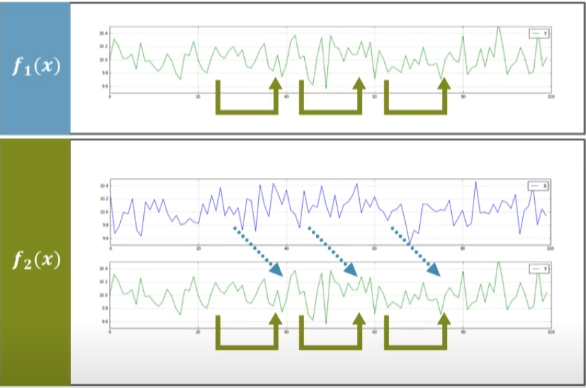
Suppose we have two cases. One is the model with one time series data that uses only past $Y$ values to predict future $Y$ values, and the other is complex model that uses not only past $Y$ but also $X$ values for prediction. In this case, the RSS (Residual Sum of Squares for short), the error can be expressed like this,

• $RSS_1 = \sum_{i=1}^n(y_i - f_1(x_i))^2$
• $RSS_2 = \sum_{i=1}^n(y_i - f_2(x_i))^2$

Of course, the error of second one(the complex one) will be smaller than first one. But is the second model the better model?

Before dealing with this problem, we bring the concept of “Degree of Freedom”(DoF for short) to express the complexity of a model. The degree of freedom is the total number of data minus the number of parameters of the model. So we can also express the degree of freedom for each model

• $DoF_1 = n - \theta_1$
• $DoF_2 = n - \theta_2$

Using them, we can derive the new term $F$ for expressing the ratio of the amount of change in RSS divided by the ratio of change in DoF.

$$F = \frac{\frac{\vert RSS_1 - RSS_2 \vert}{RSS_2}}{\frac{\vert DoF_1 - DoF_2 \vert}{DoF_2}}$$

If this value is close to 1, it means that there is not much difference in predictive performance between the two models. If it is much greater than 1, then we can determine that this is not coincidence but that the second model has a better performance. Whole process of measuring $F$ is called F-test, which was named in honor of Ronald Fisher.

So how can we determin that there is a granger causality between $X$ and $Y$? When we predict the Y value, we can say that $X$ and $Y$ are granger causality if the $X$ affects the prediction of the $Y$ value.

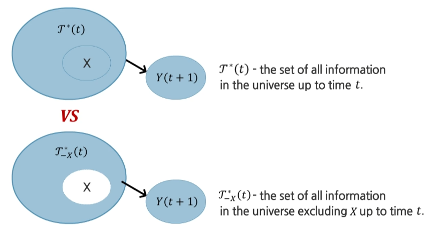
Here, we add another set to express temporal information ($\Tau$). $\Tau^(t)$ is the set of all information in the universe up to time $t$. Then, we can also define the another temporal set $\Tau_{-X}^(t)$, which is the set of all information in the universe excluding $X$ up to time $t$.

If the distribution are different like this,

$$\mathbb{P}[Y(t+1) \in A \vert \Tau^*(t)] \neq \mathbb{P}[Y(t+1) \in A \vert \Tau_{-X}^*(t)]$$

then, we can say that $X$ and $Y$ are granger causality.

Practical definition of Granger causality

We go back to previous example.

The first model uses only $Y$ for prediction, so it can be expressed like this,

$$Y_1(t) = \sum_{l=1}^L a_l Y(t - l) + \epsilon_1$$

And second model is more complex model using $X$ and $Y$ for prediction.

$$Y_2(t) = \sum_{l=1}^L a_l'Y(t-l) + \sum_{l=1}^Lb_l'X(t-l) + \epsilon_2$$

If a model using both $X$ and $Y$ has better predictive performance, it can said that $X$ and $Y$ are granger causality.

Extensive to Multivariate Time Series

Let’s look at how to determine the granger causality from the multivariate time series data by extending the existing concept. Multivariate time series is a set of time series data that contains many data within same time. From these time series, how can we know if there is a causal relationship between these various data?

Multivariate time series can be expressed like this,

$$\begin{aligned} X_i(t) &= \sum_{j=1}^p a_{i, j}^T X_j^{t, \text{lagged}} + \epsilon \\ a_{i, j} &= [a_{i, j, 1}, \dots , a_{i, j, L}] \\ X_j^{t, \text{lagged}} &= [X_j[t-L), \dots , X_j(t-1)] \end{aligned}$$

In this case, to predict the $X$ value at time $t$, a certain range of data is required from $t-1$. Here, the length of range is called lagged or window.

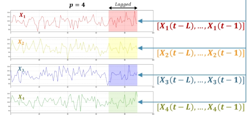
And for estimating the value at future time, it can be obtained by a linear combination of previously described values. In this case, $a$ tensor express the coefficients that multiply all time series data, which has 3 dimensions.

The two preceding dimension represent the time series data to be multiplied and the index of time series data to be predicted, And the third dimension represents the time order of the data being multiplied.

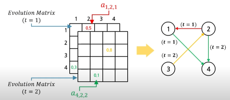
We can express it with matrix notation. Here, Evolution matrix is defined with all coefficient at time $t$. Since we use $L$ times of data, $L$ matrices are generated. If we use sparse modeling when creating a linear regression model, the element values of matrix will be mostly zero. In that case, nonzero elements represent the correlation between the two $X$ data. In other words, it helps to predict the first time series data value at time $t$.

As a result, through evolution matrix, we can interpret the model (interpretability). And it is philosophy of Granger Causality that causality always occurs in temporal order, and causes precede effects.

Summary

In this post, we can use the granger causality as a kind of temporal causality. We can also determine if there is a Granger causality by determining whether the existence of timeseries data helps to predict other time series data.