Causal Graphical Model
In this post, it will be explained about the causal graphical model. Especially, we will learn about bayesian networks with aspect of conditional independence and its analysis tool "D-separation". Also we will cover bayesian networks with have different characteristics compared to formal bayesian networks. This post is the summary of "Mathematical principles in Machine Learning" offered from UNIST.
Causal Graphical Model
Directed Acyclic Graph (DAG)
Graph is a visual notation of relationship among a set of nodes, or vertices, and a set of edges which connects between nodes. The expression “Directed” means that each nodes have direction. And if there is a path from a node, goes back to the starting node throught directed edges, the path is called Cyclic. Without this, it is called Directed Acyclic Graph(DAG for short)
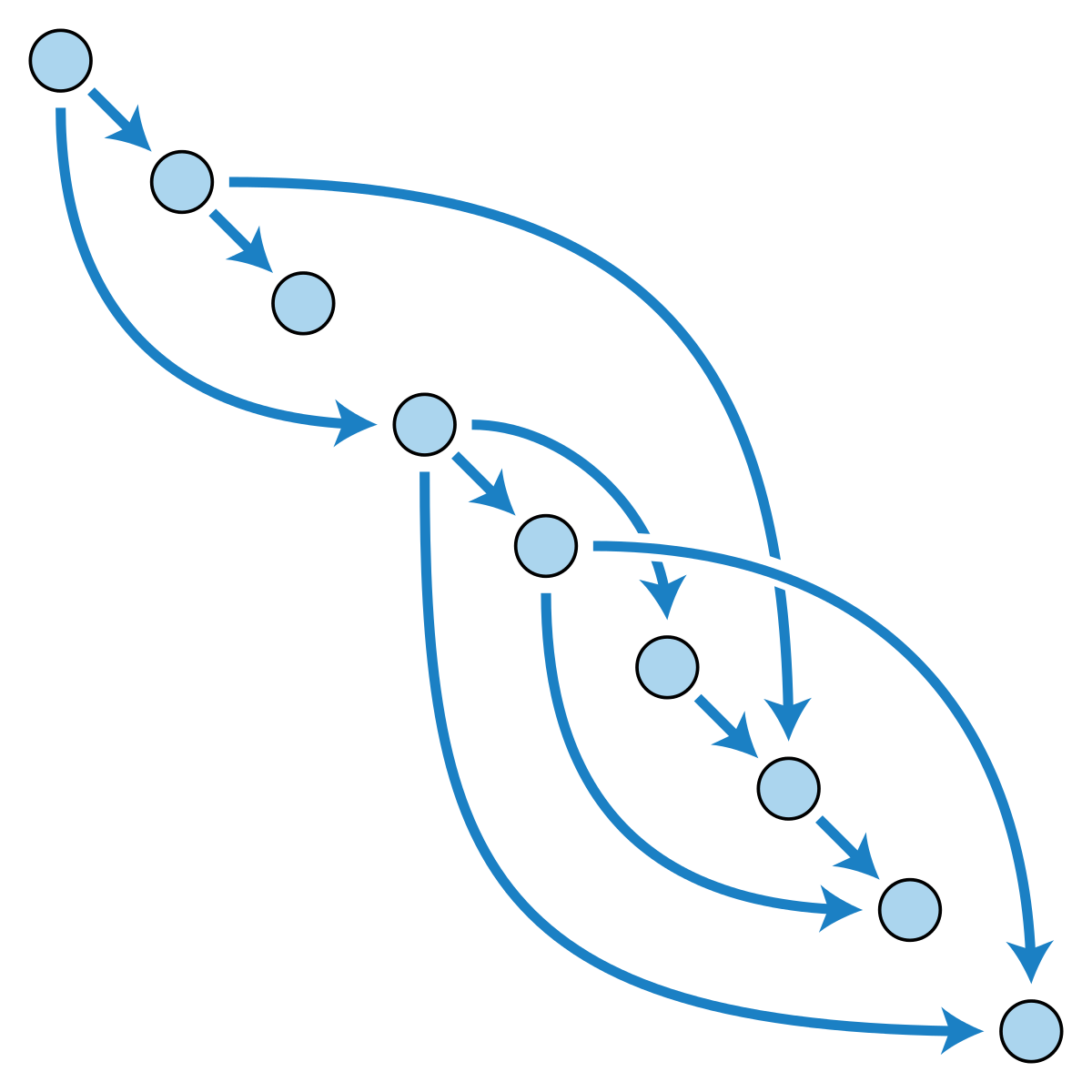
Shown in figure, there is no path to return to the starting node throught directed edges, so this is DAG. Usually, we express them with hierarchical relationship, and the node placed in higher level is called ancestor, and node in lower level is called descendant.
Conditional Dependency
Suppose we have random variable $X$ and $Y$. Its conditional probability of $X$ on $Y$ is defined as a joint probability of $X$ and $Y$ over probability of $Y$.
Here, we can assume $X$ and $Y$ are independent if these conditions are satisfied,
- $P(X \vert Y) = P(X)$
- $P(Y \vert X) = P(Y)$
- $P(X, Y) = P(X) \cdot P(Y)$
(actually those conditions are derived from the definition of conditional probability)
And it can be represented with following mathematical symbol
Let’s look at three random variables $X, Y, Z$. In this case, $X$ and $Y$ are indepedent conditioned on $Z$ if this condition is safisfied,
Bayesian Networks
Why should we review the concept of DAG and conditional probabilities? That’s because the bayesian network is implemented with DAG and have specific properties related with conditional probabilities.
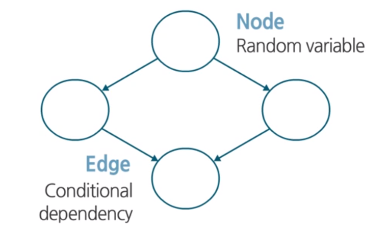
Bayesian Networks is structured, graphical representation of probabilistic relationships between several random variables. Here, Nodes represent random variables and edges between nodes represent conditional dependency.

We can draw the conditional probability table of each states. Using this, we calculates the probabilty of future states, like “What is probability of Grass Wet when it is raining and sprinkler is working?”. As shown in the example, the bayesian networks can represent a set of variables and their conditional dependence via a DAG. We can also think about the conditional independence. In this bayesian network.
As a result, the joint probability can be factorized based on the conditional independence in the bayesian networks.
Dependency in Bayesian Network
Each nodes have the rule of either head and tail. If we have three nodes, $a, b, c$, we can define the relationship in views of rules.
Tail-to-Tail
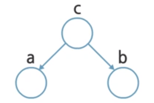
In views of $c$, $a$ and $b$ are considered to tail. So it is called Tail-to-Tail dependency.
- Joint Probability: $p(a, b, c) = p(a \vert c) p(b \vert c) p(c)$
- Independence test: $p(a, b) = \sum_c p(a \vert c) p(b \vert c) p(c) \neq p(a) p(b)$
- Notation: $a \not \perp b \vert \emptyset$
In this case, it cannot be decomposed as product of probability of $a$ and probability of $b$ in general. Therefore, $a$ and $b$ are dependent.
Head-to-Tail
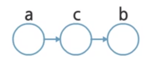
It is called Head-to-Tail dependency, since $a$ is considered as head, and $b$ is tail.
- Joint Probability: $p(a, b, c) = p(a) p(c \vert a) p(b \vert c)$
- Independence test: $p(a, b) = p(a) \sum_c p(c \vert a) p(b \vert c) = p(a) p(b \vert a) \neq p(a) p(b)$
- Notation: $a \not \perp b \vert \emptyset$
From the independence test, $a$ and $b$ are dependent, same as before.
Head-to-Head
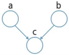
Head-to-Head dependency is a little bit different from previous case. Here, $a$ and $b$ are not conditionally dependent on any node.
- Joint Probability: $p(a, b, c) = p(a) p(b) p(c \vert a, b)$
- Independence test: $p(a, b) = p(a)p(b)
- Notation: $a \perp b \vert \emptyset$
Thus, $a$ and $b$ are independent.
What if we conditionalize $c$ by observing $c$ in all three cases?
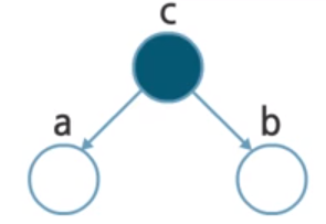
In tail-to-tail case, we can define the joint probability,
Using this, we can redo the independence test,
In this case, $a$ and $b$ are (conditionally) independent given $c$.
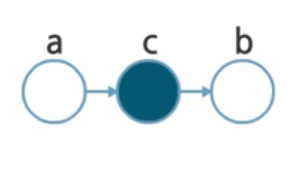
In Head-to-tail case, same process is held,
- Joint probability: $p(a, b, c) = p(a) p(c \vert a) p(b \vert c)$
- Independence test: $\begin{aligned} p(a, b \vert c) &= \frac{p(a, b, c)}{p(c)} \ &= \frac{p(a) p(c \vert a) p(b \vert c)}{p(c)} = p(a \vert c) p(b \vert c) \end{aligned}$
Same as before, $a$ and $b$ are conditionally independent given $c$.
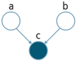
In contrast of previous cases, head-to-head case $a$ and $b$ are not conditionally independent on $c$.
- Joint probability: $p(a, b, c) = p(a) p(b) p(c \vert a, b)$
- Independence test: $\begin{aligned} p(a, b \vert c) &= \frac{p(a, b, c)}{p(c)} \ &= \frac{p(a) p(b) p(c \vert a, b)}{p(c)} \neq p(a \vert c) p(b \vert c) \end{aligned}$
- $a \not \perp b \vert c$
D-separation
From the result, if there is no connection (or path) between $a$ and $b$, A path from $a$ to $b$ is blocked. We saw the blocked cases in previous section,
- Tail-to-Tail and observed case
- Head-to-Tail and observed case
- Head-to-Head and not observed case (including its descendents)
If all paths from $a$ to $b$ is blocked by nodes in a set $C$, it is called that $a$ is D-separated from $b$ by set $C$. Here D-separation implies conditional independency.
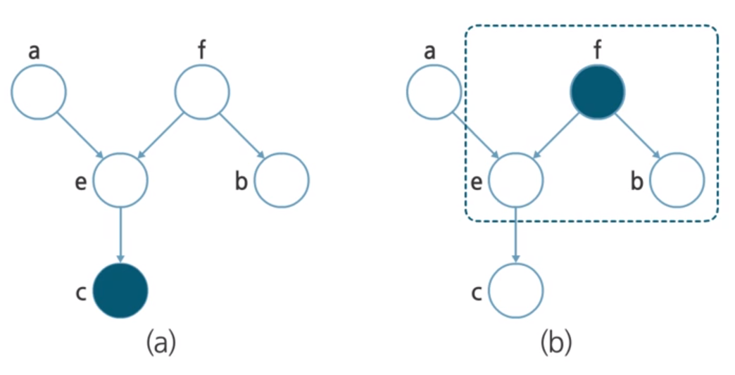
Suppose we have two simple bayesian network, and we want to know if $a$ and $b$ are conditionally independent whether $c$ is observed or not. We can simply draw the path from $a$ to $b$.
In figure (a), $c$ is observed. In this case, node $e$ shows head-to-head relation. If a node is in head-to-head relation, the node and its descendent should not be observed in order to block the path. (see the Head-to-Head blocked case). But node $c$, which is a descendent of $e$ is observed. So $e$ does not block the path.
Node $f$ is in tail-to-tail relation, but it is not observed. As it doesnot satisfy the blocking condition, it does not block the path either.
As a result, all nodes in path does not satifies the blocking condition, so the path from $a$ to $b$ is not blocked.
In figure (b), $f$ is observed. In this case, the path is blocked by $f$, as $f$ is in tail-to-tail relation and $f$ is observed, it satifies the blocking condition. So we can conclude $a$ and $b$ are conditionally independent when $f$ is observed.
Association vs. Causation
Causation implies association, but association does not necessarily imply causation, so usually conditionally probabilty rather represents association, than causation.
If we are interested in causal relations, it is more natural to represent causal relations directly.
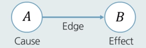
A bayesian network where each node represents a variable and the edges represent causal relations, it is called Causal Bayesian Network (CBN for short). It has stronger assumptions than bayesian networks, as all the relation should correspond to causal relations.
CBN describes the causal relationships among variables.
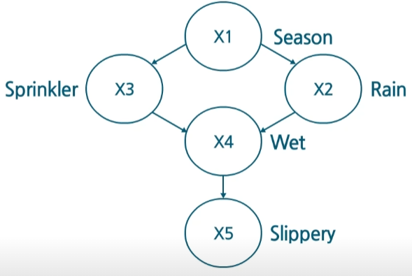
For example, It often rains as hot weather and it makes see surface temperature to elevate, therefore it makes more vapor in the air. So season is a cause of rain.
Also summer is a good time for agriculture. So we usually turn on sprinkler to make crops grow. In this case, season is cause of sprinkler.Both sprinkler and rain makes grass wet, and it makes grass to slippery.
From these causal relations, we can build a CBN. The absence of a direct link between $X_1$ and $X_5$ shows that there is no direct influence of season on slippery.
Intervention
To know the effect of something, we need to make something to change. We call it as intervention, the act of making something happen in causal model. In the previous post of Causality, we may see this notation,
Here, do operator represents the intervention, which is introduced by Judea Pearl through his book “Probabilistic Reasoning in Intelligent Systems: Networks of Plausible Inference”. In previous example, we can express the intervention like this,
So how can we use a Causal Bayesian Network for intervention? If our intervention is $do(\text{Sprinkler} = \text{on})$, then the result joint probability weill be defined in a new causal structure like this,
Note that the difference between probability conditioned on intervention and observation. Conditional probability with intervention ($P(Y \vert do(X = 1))$) is called Causal Conditioning, where an action is taken to force a specific value $x$ to know the effect of action $x$. And conditional probability with observation ($P(Y \vert X = 1)$) is called Bayesian Conditioning, where $x$ is observed variable. In this case, we don’t know if $X$ is a cause or just happening together.
In Bayesian Network, conditional probability with observation will be like this,
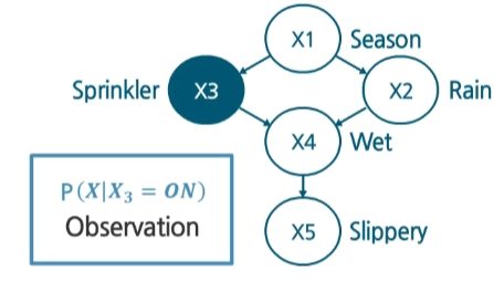
In Causal Bayesian Network, Conditional probability with intervention is,
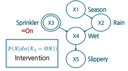
Here, it has simpler form than bayesian network since the connection between $X_3$ and $X_1$ is dropped in Causal Baysian Network. And actually $P(do(X_3 = \text{ON}) \vert x_1)$ is same as $P(do(X_3 = \text{ON}))$ so it is cancelled out. Therefore, causal bayesian network is better to infer the causal effect of each variable.
Summary
In this post, we have covered what a bayesian network is, and how to infer conditional independency using concept of D-separation. Also, we learned about causal bayesian network and its causal relationships, and how to represent intervention and infer causal effect.