Bayesian Convolutional Neural Network
In this post, we will create a Bayesian convolutional neural network to classify the famous MNIST handwritten digits. This will be a probabilistic model, designed to capture both aleatoric and epistemic uncertainty. You will test the uncertainty quantifications against a corrupted version of the dataset. This is the assignment of lecture "Probabilistic Deep Learning with Tensorflow 2" from Imperial College London.


import tensorflow as tf
import tensorflow_probability as tfp

from tensorflow.keras.models import Sequential
from tensorflow.keras.layers import Dense, Flatten, Conv2D, MaxPooling2D
from tensorflow.keras.losses import SparseCategoricalCrossentropy
from tensorflow.keras.optimizers import RMSprop

import numpy as np
import os
import matplotlib.pyplot as plt

tfd = tfp.distributions
tfpl = tfp.layers

plt.rcParams['figure.figsize'] = (10, 6)
print("Tensorflow Version: ", tf.__version__)
print("Tensorflow Probability Version: ", tfp.__version__)
The MNIST and MNIST-C datasets
In this notebook, you will use the MNIST and MNIST-C datasets, which both consist of a training set of 60,000 handwritten digits with corresponding labels, and a test set of 10,000 images. The images have been normalised and centred. The MNIST-C dataset is a corrupted version of the MNIST dataset, to test out-of-distribution robustness of computer vision models.
- Y. LeCun, L. Bottou, Y. Bengio, and P. Haffner. "Gradient-based learning applied to document recognition." Proceedings of the IEEE, 86(11):2278-2324, November 1998.
- N. Mu and J. Gilmeer. "MNIST-C: A Robustness Benchmark for Computer Vision" https://arxiv.org/abs/1906.02337
Our goal is to construct a neural network that classifies images of handwritten digits into one of 10 classes.
Load the datasets
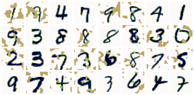
We'll start by importing two datasets. The first is the MNIST dataset of handwritten digits, and the second is the MNIST-C dataset, which is a corrupted version of the MNIST dataset. This dataset is available on TensorFlow datasets. We'll be using the dataset with "spatters". We will load and inspect the datasets below. We'll use the notation _c to denote corrupted. The images are the same as in the original MNIST, but are "corrupted" by some grey spatters.
def load_data(name):
    data_dir = os.path.join('dataset', name)
    x_train = 1 - np.load(os.path.join(data_dir, 'x_train.npy')) / 255.
    x_train = x_train.astype(np.float32)
    y_train = np.load(os.path.join(data_dir, 'y_train.npy'))
    y_train_oh = tf.keras.utils.to_categorical(y_train)
    x_test  = 1 - np.load(os.path.join(data_dir, 'x_test.npy')) / 255.
    x_test = x_test.astype(np.float32)
    y_test  = np.load(os.path.join(data_dir, 'y_test.npy'))
    y_test_oh = tf.keras.utils.to_categorical(y_test)

    return (x_train, y_train, y_train_oh), (x_test, y_test, y_test_oh)
def inspect_images(data, num_images):
    fig, ax = plt.subplots(nrows=1, ncols=num_images, figsize=(2*num_images, 2))
    for i in range(num_images):
        ax[i].imshow(data[i, ..., 0], cmap='gray')
        ax[i].axis('off')
    plt.show()
(x_train, y_train, y_train_oh), (x_test, y_test, y_test_oh) = load_data('MNIST')
inspect_images(data=x_train, num_images=8)

(x_c_train, y_c_train, y_c_train_oh), (x_c_test, y_c_test, y_c_test_oh) = load_data('MNIST_corrupted')
inspect_images(data=x_c_train, num_images=8)

def get_deterministic_model(input_shape, loss, optimizer, metrics):
    """
    This function should build and compile a CNN model according to the above specification.
    The function takes input_shape, loss, optimizer and metrics as arguments, which should be
    used to define and compile the model.
    Your function should return the compiled model.
    """
    model = Sequential([
        Conv2D(kernel_size=(5, 5), filters=8, activation='relu', padding='VALID', input_shape=input_shape),
        MaxPooling2D(pool_size=(6, 6)),
        Flatten(),
        Dense(units=10, activation='softmax')
    ])

    model.compile(loss=loss, optimizer=optimizer, metrics=metrics)
    return model
tf.random.set_seed(0)
deterministic_model = get_deterministic_model(
    input_shape=(28, 28, 1),
    loss=SparseCategoricalCrossentropy(),
    optimizer=RMSprop(),
    metrics=['accuracy']
)
deterministic_model.summary()
deterministic_model.fit(x_train, y_train, epochs=5)
print('Accuracy on MNIST test set: ',
      str(deterministic_model.evaluate(x_test, y_test, verbose=False)[1]))
print('Accuracy on corrupted MNIST test set: ',
      str(deterministic_model.evaluate(x_c_test, y_c_test, verbose=False)[1]))
As you might expect, the pointwise performance on the corrupted MNIST set is worse. This makes sense, since this dataset is slightly different, and noisier, than the uncorrupted version. Furthermore, the model was trained on the uncorrupted MNIST data, so has no experience with the spatters.
Probabilistic CNN model
You'll start by turning this deterministic network into a probabilistic one, by letting the model output a distribution instead of a deterministic tensor. This model will capture the aleatoric uncertainty on the image labels. You will do this by adding a probabilistic layer to the end of the model and training using the negative loglikelihood.
Note that, our NLL loss function has arguments y_true for the correct label (as a one-hot vector), and y_pred as the model prediction (a OneHotCategorical distribution). It should return the negative log-likelihood of each sample in y_true given the predicted distribution y_pred. If y_true is of shape [B, E] and y_pred has batch shape [B] and event shape [E], the output should be a Tensor of shape [B].
def nll(y_true, y_pred):
    """
    This function should return the negative log-likelihood of each sample
    in y_true given the predicted distribution y_pred. If y_true is of shape
    [B, E] and y_pred has batch shape [B] and event_shape [E], the output
    should be a Tensor of shape [B].
    """
    return -y_pred.log_prob(y_true)
Now we need to build probabilistic model.
def get_probabilistic_model(input_shape, loss, optimizer, metrics):
    """
    This function should return the probabilistic model according to the
    above specification.
    The function takes input_shape, loss, optimizer and metrics as arguments, which should be
    used to define and compile the model.
    Your function should return the compiled model.
    """
    model = Sequential([
        Conv2D(kernel_size=(5, 5), filters=8, activation='relu', padding='VALID', input_shape=input_shape),
        MaxPooling2D(pool_size=(6, 6)),
        Flatten(),
        Dense(tfpl.OneHotCategorical.params_size(10)),
        tfpl.OneHotCategorical(10, convert_to_tensor_fn=tfd.Distribution.mode)
    ])

    model.compile(loss=loss, optimizer=optimizer, metrics=metrics)
    return model
tf.random.set_seed(0)
probabilistic_model = get_probabilistic_model(
    input_shape=(28, 28, 1),
    loss=nll,
    optimizer=RMSprop(),
    metrics=['accuracy']
)
probabilistic_model.summary()
Now, you can train the probabilistic model on the MNIST data using the code below.
Note that the target data now uses the one-hot version of the labels, instead of the sparse version. This is to match the categorical distribution you added at the end.
probabilistic_model.fit(x_train, y_train_oh, epochs=5)
print('Accuracy on MNIST test set: ',
      str(probabilistic_model.evaluate(x_test, y_test_oh, verbose=False)[1]))
print('Accuracy on corrupted MNIST test set: ',
      str(probabilistic_model.evaluate(x_c_test, y_c_test_oh, verbose=False)[1]))
def analyse_model_prediction(data, true_labels, model, image_num, run_ensemble=False):
    if run_ensemble:
        ensemble_size = 200
    else:
        ensemble_size = 1
    image = data[image_num]
    true_label = true_labels[image_num, 0]
    predicted_probabilities = np.empty(shape=(ensemble_size, 10))
    for i in range(ensemble_size):
        predicted_probabilities[i] = model(image[np.newaxis, :]).mean().numpy()[0]
    model_prediction = model(image[np.newaxis, :])
    fig, (ax1, ax2) = plt.subplots(nrows=1, ncols=2, figsize=(10, 2),
                                   gridspec_kw={'width_ratios': [2, 4]})

    # Show the image and the true label
    ax1.imshow(image[..., 0], cmap='gray')
    ax1.axis('off')
    ax1.set_title('True label: {}'.format(str(true_label)))

    # Show a 95% prediction interval of model predicted probabilities
    pct_2p5 = np.array([np.percentile(predicted_probabilities[:, i], 2.5) for i in range(10)])
    pct_97p5 = np.array([np.percentile(predicted_probabilities[:, i], 97.5) for i in range(10)])
    bar = ax2.bar(np.arange(10), pct_97p5, color='red')
    bar[int(true_label)].set_color('green')
    ax2.bar(np.arange(10), pct_2p5-0.02, color='white', linewidth=1, edgecolor='white')
    ax2.set_xticks(np.arange(10))
    ax2.set_ylim([0, 1])
    ax2.set_ylabel('Probability')
    ax2.set_title('Model estimated probabilities')
    plt.show()
for i in [0, 1577]:
    analyse_model_prediction(x_test, y_test, probabilistic_model, i)


The model is very confident that the first image is a 6, which is correct. For the second image, the model struggles, assigning nonzero probabilities to many different classes.
Run the code below to do the same for 2 images from the corrupted MNIST test set.
for i in [0, 3710]:
    analyse_model_prediction(x_c_test, y_c_test, probabilistic_model, i)


The first is the same 6 as you saw above, but the second image is different. Notice how the model can still say with high certainty that the first image is a 6, but struggles for the second, assigning an almost uniform distribution to all possible labels.
Finally, have a look at an image for which the model is very sure on MNIST data but very unsure on corrupted MNIST data:
for i in [9241]:
    analyse_model_prediction(x_test, y_test, probabilistic_model, i)
    analyse_model_prediction(x_c_test, y_c_test, probabilistic_model, i)


It's not surprising what's happening here: the spatters cover up most of the number. You would hope a model indicates that it's unsure here, since there's very little information to go by. This is exactly what's happened.
Uncertainty quantification using entropy
We can also make some analysis of the model's uncertainty across the full test set, instead of for individual values. One way to do this is to calculate the entropy of the distribution. The entropy is the expected information (or informally, the expected 'surprise') of a random variable, and is a measure of the uncertainty of the random variable. The entropy of the estimated probabilities for sample $i$ is defined as
$$ H_i = -\sum_{j=1}^{10} p_{ij} \text{log}_{2}(p_{ij}) $$where $p_{ij}$ is the probability that the model assigns to sample $i$ corresponding to label $j$. The entropy as above is measured in bits. If the natural logarithm is used instead, the entropy is measured in nats.
The key point is that the higher the value, the more unsure the model is. Let's see the distribution of the entropy of the model's predictions across the MNIST and corrupted MNIST test sets. The plots will be split between predictions the model gets correct and incorrect.
# split into whether the model prediction is correct or incorrect


def get_correct_indices(model, x, labels):
    y_model = model(x)
    correct = np.argmax(y_model.mean(), axis=1) == np.squeeze(labels)
    correct_indices = [i for i in range(x.shape[0]) if correct[i]]
    incorrect_indices = [i for i in range(x.shape[0]) if not correct[i]]
    return correct_indices, incorrect_indices


def plot_entropy_distribution(model, x, labels):
    probs = model(x).mean().numpy()
    entropy = -np.sum(probs * np.log2(probs), axis=1)
    fig, axes = plt.subplots(1, 2, figsize=(10, 4))
    for i, category in zip(range(2), ['Correct', 'Incorrect']):
        entropy_category = entropy[get_correct_indices(model, x, labels)[i]]
        mean_entropy = np.mean(entropy_category)
        num_samples = entropy_category.shape[0]
        title = category + 'ly labelled ({:.1f}% of total)'.format(num_samples / x.shape[0] * 100)
        axes[i].hist(entropy_category, weights=(1/num_samples)*np.ones(num_samples))
        axes[i].annotate('Mean: {:.3f} bits'.format(mean_entropy), (0.4, 0.9), ha='center')
        axes[i].set_xlabel('Entropy (bits)')
        axes[i].set_ylim([0, 1])
        axes[i].set_ylabel('Probability')
        axes[i].set_title(title)
    plt.show()
print('MNIST test set:')
plot_entropy_distribution(probabilistic_model, x_test, y_test)

print('Corrupted MNIST test set:')
plot_entropy_distribution(probabilistic_model, x_c_test, y_c_test)

There are two main conclusions:
- The model is more unsure on the predictions it got wrong: this means it "knows" when the prediction may be wrong.
- The model is more unsure for the corrupted MNIST test than for the uncorrupted version. Futhermore, this is more pronounced for correct predictions than for those it labels incorrectly.
In this way, the model seems to "know" when it is unsure. This is a great property to have in a machine learning model, and is one of the advantages of probabilistic modelling.
Bayesian CNN model
The probabilistic model you just created considered only aleatoric uncertainty, assigning probabilities to each image instead of deterministic labels. The model still had deterministic weights. However, as you've seen, there is also 'epistemic' uncertainty over the weights, due to uncertainty about the parameters that explain the training data.
def get_convolutional_reparameterization_layer(input_shape, divergence_fn):
    """
    This function should create an instance of a Convolution2DReparameterization
    layer according to the above specification.
    The function takes the input_shape and divergence_fn as arguments, which should
    be used to define the layer.
    Your function should then return the layer instance.
    """

    layer = tfpl.Convolution2DReparameterization(
                input_shape=input_shape, filters=8, kernel_size=(5, 5),
                activation='relu', padding='VALID',
                kernel_prior_fn=tfpl.default_multivariate_normal_fn,
                kernel_posterior_fn=tfpl.default_mean_field_normal_fn(is_singular=False),
                kernel_divergence_fn=divergence_fn,
                bias_prior_fn=tfpl.default_multivariate_normal_fn,
                bias_posterior_fn=tfpl.default_mean_field_normal_fn(is_singular=False),
                bias_divergence_fn=divergence_fn
            )
    return layer
Custom prior
For the parameters of the DenseVariational layer, we will use a custom prior: the "spike and slab" (also called a scale mixture prior) distribution. This distribution has a density that is the weighted sum of two normally distributed ones: one with a standard deviation of 1 and one with a standard deviation of 10. In this way, it has a sharp spike around 0 (from the normal distribution with standard deviation 1), but is also more spread out towards far away values (from the contribution from the normal distribution with standard deviation 10). The reason for using such a prior is that it is like a standard unit normal, but makes values far away from 0 more likely, allowing the model to explore a larger weight space. Run the code below to create a "spike and slab" distribution and plot its probability density function, compared with a standard unit normal.
def spike_and_slab(event_shape, dtype):
    distribution = tfd.Mixture(
        cat=tfd.Categorical(probs=[0.5, 0.5]),
        components=[
            tfd.Independent(tfd.Normal(
                loc=tf.zeros(event_shape, dtype=dtype),
                scale=1.0*tf.ones(event_shape, dtype=dtype)),
                            reinterpreted_batch_ndims=1),
            tfd.Independent(tfd.Normal(
                loc=tf.zeros(event_shape, dtype=dtype),
                scale=10.0*tf.ones(event_shape, dtype=dtype)),
                            reinterpreted_batch_ndims=1)],
    name='spike_and_slab')
    return distribution
x_plot = np.linspace(-5, 5, 1000)[:, np.newaxis]
plt.plot(x_plot, tfd.Normal(loc=0, scale=1).prob(x_plot).numpy(), label='unit normal', linestyle='--')
plt.plot(x_plot, spike_and_slab(1, dtype=tf.float32).prob(x_plot).numpy(), label='spike and slab')
plt.xlabel('x')
plt.ylabel('Density')
plt.legend()
plt.show()

def get_prior(kernel_size, bias_size, dtype=None):
    """
    This function should create the prior distribution, consisting of the
    "spike and slab" distribution that is described above.
    The distribution should be created using the kernel_size, bias_size and dtype
    function arguments above.
    The function should then return a callable, that returns the prior distribution.
    """
    n = kernel_size+bias_size
    prior_model = Sequential([tfpl.DistributionLambda(lambda t : spike_and_slab(n, dtype))])
    return prior_model
def get_posterior(kernel_size, bias_size, dtype=None):
    """
    This function should create the posterior distribution as specified above.
    The distribution should be created using the kernel_size, bias_size and dtype
    function arguments above.
    The function should then return a callable, that returns the posterior distribution.
    """
    n = kernel_size + bias_size
    return Sequential([
        tfpl.VariableLayer(tfpl.IndependentNormal.params_size(n), dtype=dtype),
        tfpl.IndependentNormal(n)
    ])
def get_dense_variational_layer(prior_fn, posterior_fn, kl_weight):
    """
    This function should create an instance of a DenseVariational layer according
    to the above specification.
    The function takes the prior_fn, posterior_fn and kl_weight as arguments, which should
    be used to define the layer.
    Your function should then return the layer instance.
    """
    return tfpl.DenseVariational(
        units=10, make_posterior_fn=posterior_fn, make_prior_fn=prior_fn, kl_weight=kl_weight
    )
Now, you're ready to use the functions you defined to create the convolutional reparameterization and dense variational layers, and use them in your Bayesian convolutional neural network model.
tf.random.set_seed(0)
divergence_fn = lambda q, p, _ : tfd.kl_divergence(q, p) / x_train.shape[0]
convolutional_reparameterization_layer = get_convolutional_reparameterization_layer(
    input_shape=(28, 28, 1), divergence_fn=divergence_fn
)
dense_variational_layer = get_dense_variational_layer(
    get_prior, get_posterior, kl_weight=1/x_train.shape[0]
)
bayesian_model = Sequential([
    convolutional_reparameterization_layer,
    MaxPooling2D(pool_size=(6, 6)),
    Flatten(),
    dense_variational_layer,
    tfpl.OneHotCategorical(10, convert_to_tensor_fn=tfd.Distribution.mode)
])
bayesian_model.compile(loss=nll,
              optimizer=RMSprop(),
              metrics=['accuracy'],
              experimental_run_tf_function=False)
bayesian_model.summary()
bayesian_model.fit(x=x_train, y=y_train_oh, epochs=10, verbose=True)
print('Accuracy on MNIST test set: ',
      str(bayesian_model.evaluate(x_test, y_test_oh, verbose=False)[1]))
print('Accuracy on corrupted MNIST test set: ',
      str(bayesian_model.evaluate(x_c_test, y_c_test_oh, verbose=False)[1]))
Analyse the model predictions
Now that the model has trained, run the code below to create the same plots as before, starting with an analysis of the predicted probabilities for the same images.
This model now has weight uncertainty, so running the forward pass multiple times will not generate the same estimated probabilities. For this reason, the estimated probabilities do not have single values. The plots are adjusted to show a 95% prediction interval for the model's estimated probabilities.
for i in [0, 1577]:
    analyse_model_prediction(x_test, y_test, bayesian_model, i, run_ensemble=True)


For the first image, the model assigns a probability of almost one for the 6 label. Furthermore, it is confident in this probability: this probability remains close to one for every sample from the posterior weight distribution (as seen by the horizontal green line having very small height, indicating a narrow prediction interval). This means that the epistemic uncertainty on this probability is very low.
For the second image, the epistemic uncertainty on the probabilities is much larger, which indicates that the estimated probabilities may be unreliable. In this way, the model indicates whether estimates may be inaccurate.
for i in [0, 3710]:
    analyse_model_prediction(x_c_test, y_c_test, bayesian_model, i, run_ensemble=True)


Even with the spatters, the Bayesian model is confident in predicting the correct label for the first image above. The model struggles with the second image, which is reflected in the range of probabilities output by the network.
for i in [9241]:
    analyse_model_prediction(x_test, y_test, bayesian_model, i, run_ensemble=True)
    analyse_model_prediction(x_c_test, y_c_test, bayesian_model, i, run_ensemble=True)


Similar to before, the model struggles with the second number, as it is mostly covered up by the spatters. However, this time is clear to see the epistemic uncertainty in the model.
print('MNIST test set:')
plot_entropy_distribution(bayesian_model, x_test, y_test)

print('Corrupted MNIST test set:')
plot_entropy_distribution(bayesian_model, x_c_test, y_c_test)
