RealNVP for the LSUN bedroom dataset
In this post, we are take a look at an application for RealNVP. This is a homework assignment of lecture "Probabilistic Deep Learning with Tensorflow 2" from Imperial College London.


- Packages
- The LSUN Bedroom Dataset
- Load the dataset
- Binary masks
- Combining the affine coupling layers
- Multiscale architecture
- Data preprocessing bijector
- Train the RealNVP model
- Generate some samples
import tensorflow as tf
import tensorflow_probability as tfp

import numpy as np
import matplotlib.pyplot as plt

tfd = tfp.distributions
tfpl = tfp.layers
tfb = tfp.bijectors

plt.rcParams['figure.figsize'] = (10, 6)
print("Tensorflow Version: ", tf.__version__)
print("Tensorflow Probability Version: ", tfp.__version__)
The LSUN Bedroom Dataset
In this post, you will use a subset of the LSUN dataset. This is a large-scale image dataset with 10 scene and 20 object categories. A subset of the LSUN bedroom dataset has been provided, and has already been downsampled and preprocessed into smaller, fixed-size images.
- F. Yu, A. Seff, Y. Zhang, S. Song, T. Funkhouser and J. Xia. "LSUN: Construction of a Large-scale Image Dataset using Deep Learning with Humans in the Loop". arXiv:1506.03365, 10 Jun 2015
Our goal is to develop the RealNVP normalising flow architecture using bijector subclassing, and use it to train a generative model of the LSUN bedroom data subset. For full details on the RealNVP model, refer to the original paper:
- L. Dinh, J. Sohl-Dickstein and S. Bengio. "Density estimation using Real NVP". arXiv:1605.08803, 27 Feb 2017.
Load the dataset
The following functions will be useful for loading and preprocessing the dataset. The subset you will use for this assignment consists of 10,000 training images, 1000 validation images and 1000 test images.
The images have been downsampled to 32 x 32 x 3 in order to simplify the training process.
def load_image(img):
    img = tf.image.random_flip_left_right(img)
    return img, img

def load_dataset(split):
    train_list_ds = tf.data.Dataset.from_tensor_slices(np.load('./dataset/lsun/{}.npy'.format(split)))
    train_ds = train_list_ds.map(load_image)
    return train_ds
train_ds = load_dataset('train')
val_ds = load_dataset('val')
test_ds = load_dataset('test')
shuffle_buffer_size = 1000
train_ds = train_ds.shuffle(shuffle_buffer_size)
val_ds = val_ds.shuffle(shuffle_buffer_size)
test_ds = test_ds.shuffle(shuffle_buffer_size)
n_img = 4
f, axs = plt.subplots(n_img, n_img, figsize=(14, 14))

for k, image in enumerate(train_ds.take(n_img**2)):
    i = k // n_img
    j = k % n_img
    axs[i, j].imshow(image[0])
    axs[i, j].axis('off')
f.subplots_adjust(wspace=0.01, hspace=0.03)

batch_size = 64
train_ds = train_ds.batch(batch_size)
val_ds = val_ds.batch(batch_size)
test_ds = test_ds.batch(batch_size)
Affine coupling layer
We will begin the development of the RealNVP architecture with the core bijector that is called the affine coupling layer. This bijector can be described as follows: suppose that $x$ is a $D$-dimensional input, and let $d<D$. Then the output $y$ of the affine coupling layer is given by the following equations:
$$ \begin{aligned} y_{1:d} &= x_{1:d} \qquad \text{(1)} \\ y_{d+1:D} &= x_{d+1:D}\odot \exp(s(x_{1:d})) + t(x_{1:d}), \qquad \text{(2)} \end{aligned} $$where $s$ and $t$ are functions from $\mathbb{R}^d\rightarrow\mathbb{R}^{D-d}$, and define the log-scale and shift operations on the vector $x_{d+1:D}$ respectively.
The log of the Jacobian determinant for this layer is given by $\sum_{j}s(x_{1:d})_j$.
The inverse operation can be easily computed as
$$ \begin{aligned} x_{1:d} &= y_{1:d} \qquad \text{(3)}\\ x_{d+1:D} &= \left(y_{d+1:D} - t(y_{1:d})\right)\odot \exp(-s(y_{1:d})),\qquad \text{(4)} \end{aligned} $$In practice, we will implement equations $(1)$ and $(2)$ using a binary mask $b$:
$$ \begin{aligned} \text{Forward pass:}\qquad y &= b\odot x + (1-b)\odot\left(x\odot\exp(s(b\odot x)) + t(b\odot x)\right),\qquad \text{(5)}\\ \text{Inverse pass:}\qquad x &= b\odot y + (1-b)\odot\left(y - t(b\odot x)) \odot\exp( -s(b\odot x)\right).\qquad \text{(6)} \end{aligned} $$Our inputs $x$ will be a batch of 3-dimensional Tensors with height, width and channels dimensions. As in the original architecture, we will use both spatial 'checkerboard' masks and channel-wise masks:
from tensorflow.keras import Input
from tensorflow.keras.models import Model
from tensorflow.keras.layers import Conv2D, BatchNormalization
from tensorflow.keras.regularizers import l2
from tensorflow.keras.optimizers import Adam
def get_conv_resnet(input_shape, filters):
    """
    This function should build a CNN ResNet model according to the above specification,
    using the functional API. The function takes input_shape as an argument, which should be
    used to specify the shape in the Input layer, as well as a filters argument, which
    should be used to specify the number of filters in (some of) the convolutional layers.
    Your function should return the model.
    """
    h0 = Input(shape=input_shape)

    # 1st Skip connection
    y = Conv2D(filters=filters, kernel_size=3, padding='SAME', activation='relu', kernel_regularizer=l2(l=5e-5))(h0)
    y = BatchNormalization()(y)
    y = Conv2D(filters=input_shape[-1], kernel_size=3, padding='SAME', activation='relu', kernel_regularizer=l2(l=5e-5))(y)
    y = BatchNormalization()(y)
    h1 = tf.math.add(y, h0)

    # 2nd skip connection
    y = Conv2D(filters=filters, kernel_size=3, padding='SAME', activation='relu', kernel_regularizer=l2(l=5e-5))(h1)
    y = BatchNormalization()(y)
    y = Conv2D(filters=input_shape[-1], kernel_size=3, padding='SAME', activation='relu', kernel_regularizer=l2(l=5e-5))(y)
    y = BatchNormalization()(y)
    y = tf.math.add(y, h1)
    h2 = Conv2D(filters=2 * input_shape[-1], kernel_size=3, padding='SAME', activation='linear', kernel_regularizer=l2(l=5e-5))(y)
    shift, log_scale = tf.split(h2, num_or_size_splits=2, axis=-1)
    y = tf.math.tanh(log_scale)
    model = Model(inputs=h0, outputs=[shift, y])
    return model
conv_resnet = get_conv_resnet((32, 32, 3), 32)
conv_resnet.summary()
tf.keras.utils.plot_model(conv_resnet, show_layer_names=False, rankdir='LR')

print(conv_resnet(tf.random.normal((1, 32, 32, 3)))[0].shape)
print(conv_resnet(tf.random.normal((1, 32, 32, 3)))[1].shape)
Binary masks
Now that you have a shift and log-scale model built, we will now implement the affine coupling layer. We will first need functions to create the binary masks $b$ as described above. The following function creates the spatial 'checkerboard' mask.
It takes a rank-2 shape as input, which correspond to the height and width dimensions, as well as an orientation argument (an integer equal to 0 or 1) that determines which way round the zeros and ones are entered into the Tensor.
def checkerboard_binary_mask(shape, orientation=0):
    height, width = shape[0], shape[1]
    height_range = tf.range(height)
    width_range = tf.range(width)
    height_odd_inx = tf.cast(tf.math.mod(height_range, 2), dtype=tf.bool)
    width_odd_inx = tf.cast(tf.math.mod(width_range, 2), dtype=tf.bool)
    odd_rows = tf.tile(tf.expand_dims(height_odd_inx, -1), [1, width])
    odd_cols = tf.tile(tf.expand_dims(width_odd_inx, 0), [height, 1])
    checkerboard_mask = tf.math.logical_xor(odd_rows, odd_cols)
    if orientation == 1:
        checkerboard_mask = tf.math.logical_not(checkerboard_mask)
    return tf.cast(tf.expand_dims(checkerboard_mask, -1), tf.float32)
This function creates a rank-3 Tensor to mask the height, width and channels dimensions of the input. We can take a look at this checkerboard mask for some example inputs below. In order to make the Tensors easier to inspect, we will squeeze out the single channel dimension (which is always 1 for this mask).
# NB: we squeeze the shape for easier viewing. The full shape is (4, 4, 1)

tf.squeeze(checkerboard_binary_mask((4, 4), orientation=0))
tf.squeeze(checkerboard_binary_mask((4, 4), orientation=1))
def channel_binary_mask(num_channels, orientation=0):
    """
    This function takes an integer num_channels and orientation (0 or 1) as
    arguments. It should create a channel-wise binary mask with
    dtype=tf.float32, according to the above specification.
    The function should then return the binary mask.
    """
    mask_list = []

    for i in range(num_channels):
        if i < num_channels // 2:
            mask_list.append(orientation)
        else:
            mask_list.append(not orientation)

    mask = tf.cast(tf.constant(np.array([[mask_list]])),dtype=tf.float32)
    return mask
channel_binary_mask(6, orientation=0)
def forward(x, b, shift_and_log_scale_fn):
    """
    This function takes the input Tensor x, binary mask b and callable
    shift_and_log_scale_fn as arguments.
    This function should implement the forward transformation in equation (5)
    and return the output Tensor y, which will have the same shape as x
    """
    x_b = x * b
    shift, log_scale = shift_and_log_scale_fn(x_b)
    y = x_b + (1 - b) * (x * tf.math.exp(log_scale) + shift)
    return y

def inverse(y, b, shift_and_log_scale_fn):
    """
    This function takes the input Tensor x, binary mask b and callable
    shift_and_log_scale_fn as arguments.
    This function should implement the forward transformation in equation (6)
    and return the output Tensor y, which will have the same shape as x
    """
    y_b = y * b
    shift, log_scale = shift_and_log_scale_fn(y_b)
    x = y_b + (1 - b) * (y - shift) * tf.math.exp(-log_scale)
    return x
The new bijector class also requires the log_det_jacobian methods to be implemented. Recall that the log of the Jacobian determinant of the forward transformation is given by $\sum_{j}s(x_{1:d})_j$, where $s$ is the log-scale function of the affine coupling layer.
def forward_log_det_jacobian(x, b, shift_and_log_scale_fn):
    """
    This function takes the input Tensor x, binary mask b and callable
    shift_and_log_scale_fn as arguments.
    This function should compute and return the log of the Jacobian determinant
    of the forward transformation in equation (5)
    """
    x_b = x * b
    shift, log_scale = shift_and_log_scale_fn(x_b)
    return tf.reduce_sum(log_scale * (1 - b), [1, 2, 3])


def inverse_log_det_jacobian(y, b, shift_and_log_scale_fn):
    """
    This function takes the input Tensor y, binary mask b and callable
    shift_and_log_scale_fn as arguments.
    This function should compute and return the log of the Jacobian determinant
    of the forward transformation in equation (6)
    """
    y_b = y * b
    shift, log_scale = shift_and_log_scale_fn(y_b)
    return tf.reduce_sum(-log_scale * (1 - b), [1, 2, 3])
class AffineCouplingLayer(tfb.Bijector):
    """
    Class to implement the affine coupling layer.
    Complete the __init__ and _get_mask methods according to the instructions above.
    """

    def __init__(self, shift_and_log_scale_fn, mask_type, orientation, **kwargs):
        """
        The class initialiser takes the shift_and_log_scale_fn callable, mask_type,
        orientation and possibly extra keywords arguments. It should call the
        base class initialiser, passing any extra keyword arguments along.
        It should also set the required arguments as class attributes.
        """
        super(AffineCouplingLayer, self).__init__(**kwargs, forward_min_event_ndims=3)
        self.shift_and_log_scale_fn = shift_and_log_scale_fn
        self.mask_type = mask_type
        self.orientation = orientation


    def _get_mask(self, shape):
        """
        This internal method should use the binary mask functions above to compute
        and return the binary mask, according to the arguments passed in to the
        initialiser.
        """
        height, width, channels = shape[-3:]

        if self.mask_type == 'checkerboard' :
            mask = checkerboard_binary_mask((height, width), self.orientation)
        elif self.mask_type == 'channel':
            mask = channel_binary_mask(channels, self.orientation)
        return mask

    def _forward(self, x):
        b = self._get_mask(x.shape)
        return forward(x, b, self.shift_and_log_scale_fn)

    def _inverse(self, y):
        b = self._get_mask(y.shape)
        return inverse(y, b, self.shift_and_log_scale_fn)

    def _forward_log_det_jacobian(self, x):
        b = self._get_mask(x.shape)
        return forward_log_det_jacobian(x, b, self.shift_and_log_scale_fn)

    def _inverse_log_det_jacobian(self, y):
        b = self._get_mask(y.shape)
        return inverse_log_det_jacobian(y, b, self.shift_and_log_scale_fn)
affine_coupling_layer = AffineCouplingLayer(conv_resnet, 'channel', orientation=1,
                                            name='affine_coupling_layer')
affine_coupling_layer.forward(tf.random.normal((16, 32, 32, 3))).shape
affine_coupling_layer.forward_log_det_jacobian(tf.random.normal((16, 32, 32, 3)), event_ndims=3).shape
Combining the affine coupling layers
In the affine coupling layer, part of the input remains unchanged in the transformation $(5)$. In order to allow transformation of all of the input, several coupling layers are composed, with the orientation of the mask being reversed in subsequent layers.
Our model design will be similar to the original architecture; we will compose three affine coupling layers with checkerboard masking, followed by a batch normalization bijector (tfb.BatchNormalization is a built-in bijector), followed by a squeezing operation, followed by three more affine coupling layers with channel-wise masking and a final batch normalization bijector.
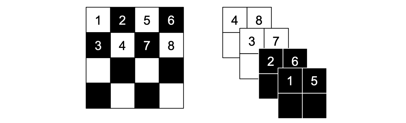
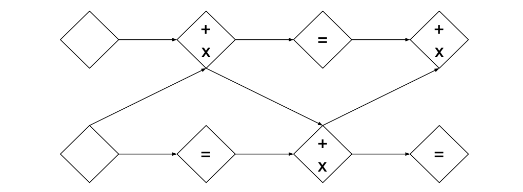
The squeezing operation divides the spatial dimensions into 2x2 squares, and reshapes a Tensor of shape (H, W, C) into a Tensor of shape (H // 2, W // 2, 4 * C) as shown in Figure 1.
The squeezing operation is also a bijective operation, and has been provided for you in the class below.
class Squeeze(tfb.Bijector):

    def __init__(self, name='Squeeze', **kwargs):
        super(Squeeze, self).__init__(forward_min_event_ndims=3, is_constant_jacobian=True,
                                      name=name, **kwargs)

    def _forward(self, x):
        input_shape = x.shape
        height, width, channels = input_shape[-3:]
        y = tfb.Reshape((height // 2, 2, width // 2, 2, channels), event_shape_in=(height, width, channels))(x)
        y = tfb.Transpose(perm=[0, 2, 1, 3, 4])(y)
        y = tfb.Reshape((height // 2, width // 2, 4 * channels),
                        event_shape_in=(height // 2, width // 2, 2, 2, channels))(y)
        return y

    def _inverse(self, y):
        input_shape = y.shape
        height, width, channels = input_shape[-3:]
        x = tfb.Reshape((height, width, 2, 2, channels // 4), event_shape_in=(height, width, channels))(y)
        x = tfb.Transpose(perm=[0, 2, 1, 3, 4])(x)
        x = tfb.Reshape((2 * height, 2 * width, channels // 4),
                        event_shape_in=(height, 2, width, 2, channels // 4))(x)
        return x

    def _forward_log_det_jacobian(self, x):
        return tf.constant(0., x.dtype)

    def _inverse_log_det_jacobian(self, y):
        return tf.constant(0., y.dtype)

    def _forward_event_shape_tensor(self, input_shape):
        height, width, channels = input_shape[-3], input_shape[-2], input_shape[-1]
        return height // 2, width // 2, 4 * channels

    def _inverse_event_shape_tensor(self, output_shape):
        height, width, channels = output_shape[-3], output_shape[-2], output_shape[-1]
        return height * 2, width * 2, channels // 4
You can see the effect of the squeezing operation on some example inputs in the cells below. In the forward transformation, each spatial dimension is halved, whilst the channel dimension is multiplied by 4. The opposite happens in the inverse transformation.
squeeze = Squeeze()
squeeze(tf.ones((10, 32, 32, 3))).shape
squeeze.inverse(tf.ones((10, 4, 4, 96))).shape
We can now construct a block of coupling layers according to the architecture described above. Our Chained bijector has specific structure,
- Three
AffineCouplingLayerbijectors with"checkerboard"masking with orientations0, 1, 0respectively - A
BatchNormalizationbijector - A
Squeezebijector - Three more
AffineCouplingLayerbijectors with"channel"masking with orientations0, 1, 0respectively - Another
BatchNormalizationbijector
The function takes the following arguments:
-
shift_and_log_scale_fns: a list or tuple of six conv_resnet models- The first three models in this list are used in the three coupling layers with checkerboard masking
- The last three models in this list are used in the three coupling layers with channel masking
-
squeeze: an instance of theSqueezebijector
def realnvp_block(shift_and_log_scale_fns, squeeze):
    """
    This function takes a list or tuple of six conv_resnet models, and an
    instance of the Squeeze bijector.
    The function should construct the chain of bijectors described above,
    using the conv_resnet models in the coupling layers.
    The function should then return the chained bijector.
    """
    bijectors = []
    orientations = [0, 1, 0]
    for i in range(3):
        bijectors.append(AffineCouplingLayer(shift_and_log_scale_fn=shift_and_log_scale_fns[i],
                                             mask_type='checkerboard',
                                             orientation=orientations[i]))
    bijectors.append(tfb.BatchNormalization())
    bijectors.append(squeeze)

    for i in range(3, 6):
        bijectors.append(AffineCouplingLayer(shift_and_log_scale_fn=shift_and_log_scale_fns[i],
                                             mask_type='channel',
                                             orientation=orientations[i % 3]))
    bijectors.append(tfb.BatchNormalization())

    flow_bijector = tfb.Chain(list(reversed(bijectors[:-1])))
    return flow_bijector
checkerboard_fns = []
for _ in range(3):
    checkerboard_fns.append(get_conv_resnet((32, 32, 3), 512))
channel_fns = []
for _ in range(3):
    channel_fns.append(get_conv_resnet((16, 16, 12), 512))

block = realnvp_block(checkerboard_fns + channel_fns, squeeze)
block.forward(tf.random.normal((10, 32, 32, 3))).shape
Multiscale architecture
The final component of the RealNVP is the multiscale architecture. The squeeze operation reduces the spatial dimensions but increases the channel dimensions. After one of the blocks of coupling-squeeze-coupling that you have implemented above, half of the dimensions are factored out as latent variables, while the other half is further processed through subsequent layers. This results in latent variables that represent different scales of features in the model.
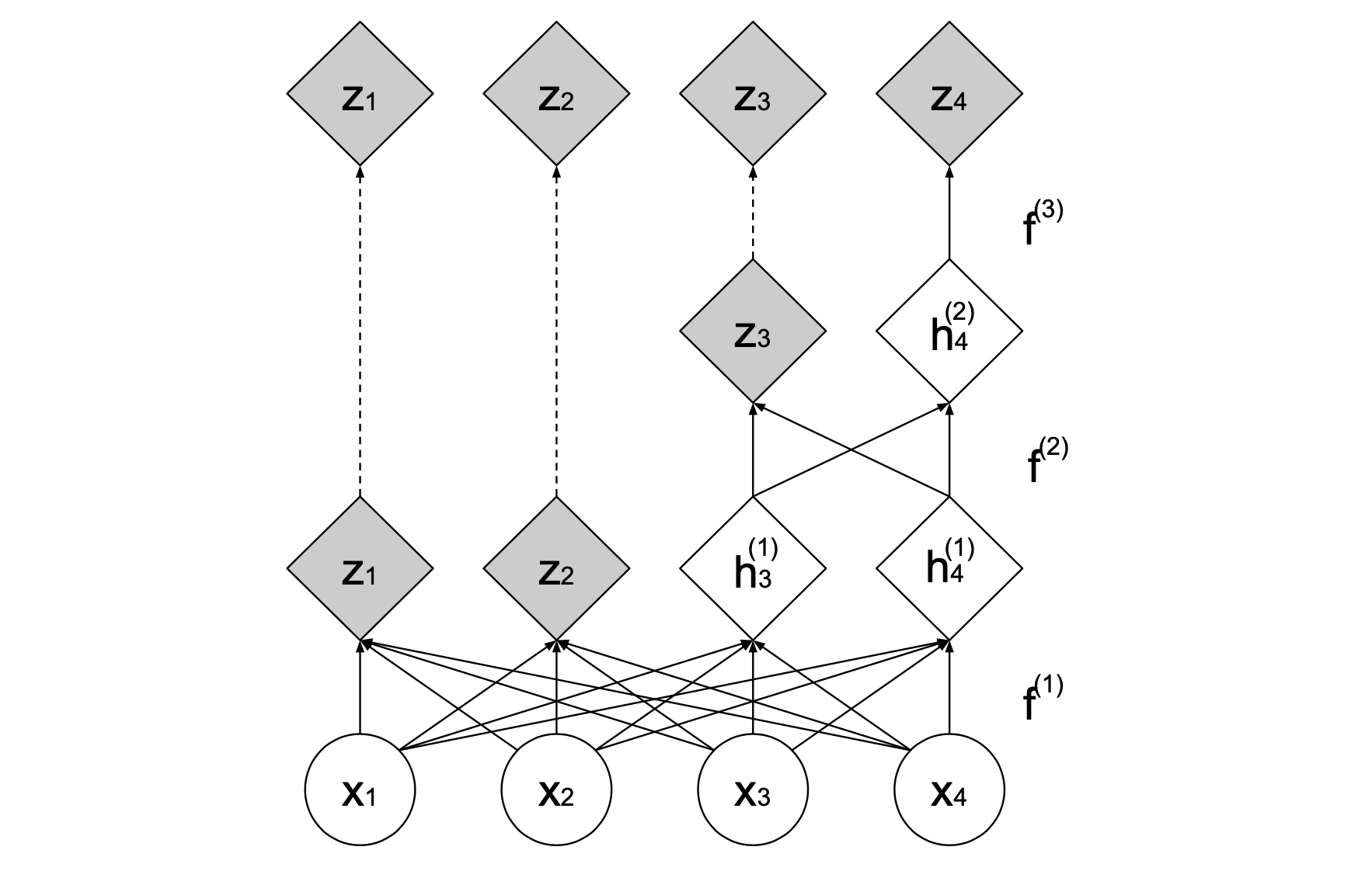
The final scale does not use the squeezing operation, and instead applies four affine coupling layers with alternating checkerboard masks.
The multiscale architecture for two latent variable scales is implemented for you in the following bijector.
class RealNVPMultiScale(tfb.Bijector):

    def __init__(self, **kwargs):
        super(RealNVPMultiScale, self).__init__(forward_min_event_ndims=3, **kwargs)

        # First level
        shape1 = (32, 32, 3)  # Input shape
        shape2 = (16, 16, 12)  # Shape after the squeeze operation
        shape3 = (16, 16, 6)  # Shape after factoring out the latent variable
        self.conv_resnet1 = get_conv_resnet(shape1, 64)
        self.conv_resnet2 = get_conv_resnet(shape1, 64)
        self.conv_resnet3 = get_conv_resnet(shape1, 64)
        self.conv_resnet4 = get_conv_resnet(shape2, 128)
        self.conv_resnet5 = get_conv_resnet(shape2, 128)
        self.conv_resnet6 = get_conv_resnet(shape2, 128)
        self.squeeze = Squeeze()
        self.block1 = realnvp_block([self.conv_resnet1, self.conv_resnet2,
                                    self.conv_resnet3, self.conv_resnet4,
                                    self.conv_resnet5, self.conv_resnet6], self.squeeze)

        # Second level
        self.conv_resnet7 = get_conv_resnet(shape3, 128)
        self.conv_resnet8 = get_conv_resnet(shape3, 128)
        self.conv_resnet9 = get_conv_resnet(shape3, 128)
        self.conv_resnet10 = get_conv_resnet(shape3, 128)
        self.coupling_layer1 = AffineCouplingLayer(self.conv_resnet7, 'checkerboard', 0)
        self.coupling_layer2 = AffineCouplingLayer(self.conv_resnet8, 'checkerboard', 1)
        self.coupling_layer3 = AffineCouplingLayer(self.conv_resnet9, 'checkerboard', 0)
        self.coupling_layer4 = AffineCouplingLayer(self.conv_resnet10, 'checkerboard', 1)
        self.block2 = tfb.Chain([self.coupling_layer4, self.coupling_layer3,
                                 self.coupling_layer2, self.coupling_layer1])

    def _forward(self, x):
        h1 = self.block1.forward(x)
        z1, h2 = tf.split(h1, 2, axis=-1)
        z2 = self.block2.forward(h2)
        return tf.concat([z1, z2], axis=-1)

    def _inverse(self, y):
        z1, z2 = tf.split(y, 2, axis=-1)
        h2 = self.block2.inverse(z2)
        h1 = tf.concat([z1, h2], axis=-1)
        return self.block1.inverse(h1)

    def _forward_log_det_jacobian(self, x):
        log_det1 = self.block1.forward_log_det_jacobian(x, event_ndims=3)
        h1 = self.block1.forward(x)
        _, h2 = tf.split(h1, 2, axis=-1)
        log_det2 = self.block2.forward_log_det_jacobian(h2, event_ndims=3)
        return log_det1 + log_det2

    def _inverse_log_det_jacobian(self, y):
        z1, z2 = tf.split(y, 2, axis=-1)
        h2 = self.block2.inverse(z2)
        log_det2 = self.block2.inverse_log_det_jacobian(z2, event_ndims=3)
        h1 = tf.concat([z1, h2], axis=-1)
        log_det1 = self.block1.inverse_log_det_jacobian(h1, event_ndims=3)
        return log_det1 + log_det2

    def _forward_event_shape_tensor(self, input_shape):
        height, width, channels = input_shape[-3], input_shape[-2], input_shape[-1]
        return height // 4, width // 4, 16 * channels

    def _inverse_event_shape_tensor(self, output_shape):
        height, width, channels = output_shape[-3], output_shape[-2], output_shape[-1]
        return 4 * height, 4 * width, channels // 16
multiscale_bijector = RealNVPMultiScale()
Data preprocessing bijector
We will also preprocess the image data before sending it through the RealNVP model. To do this, for a Tensor $x$ of pixel values in $[0, 1]^D$, we transform $x$ according to the following:
$$ T(x) = \text{logit}\left(\alpha + (1 - 2\alpha)x\right),\tag{7} $$where $\alpha$ is a parameter, and the logit function is the inverse of the sigmoid function, and is given by
$$ \text{logit}(p) = \log (p) - \log (1 - p). $$def get_preprocess_bijector(alpha):
"""
This function should create a chained bijector that computes the
transformation T in equation (7) above.
This can be computed using in-built bijectors from the bijectors module.
Your function should then return the chained bijector.
"""
return tfb.Chain([tfb.Invert(tfb.Sigmoid()), tfb.Shift(shift=alpha), tfb.Scale(scale=(1 - 2 * alpha))])
preprocess = get_preprocess_bijector(0.05)
class RealNVPModel(Model):

    def __init__(self, **kwargs):
        super(RealNVPModel, self).__init__(**kwargs)
        self.preprocess = get_preprocess_bijector(0.05)
        self.realnvp_multiscale = RealNVPMultiScale()
        self.bijector = tfb.Chain([self.realnvp_multiscale, self.preprocess])

    def build(self, input_shape):
        output_shape = self.bijector(tf.expand_dims(tf.zeros(input_shape[1:]), axis=0)).shape
        self.base = tfd.Independent(tfd.Normal(loc=tf.zeros(output_shape[1:]), scale=1.),
                                    reinterpreted_batch_ndims=3)
        self._bijector_variables = (
            list(self.bijector.variables))
        self.flow = tfd.TransformedDistribution(
            distribution=self.base,
            bijector=tfb.Invert(self.bijector),
        )
        super(RealNVPModel, self).build(input_shape)

    def call(self, inputs, training=None, **kwargs):
        return self.flow

    def sample(self, batch_size):
        sample = self.base.sample(batch_size)
        return self.bijector.inverse(sample)
realnvp_model = RealNVPModel()
realnvp_model.build((1, 32, 32, 3))
print("Total trainable variables:")
print(sum([np.prod(v.shape) for v in realnvp_model.trainable_variables]))
Note that the model's call method returns the TransformedDistribution object. Also, we have set up our datasets to return the input image twice as a 2-tuple. This is so we can train our model with negative log-likelihood as normal.
def nll(y_true, y_pred):
    return -y_pred.log_prob(y_true)
It is recommended to use the GPU accelerator hardware on Colab to train this model, as it can take some time to train. Note that it is not required to train the model in order to pass this assignment. For optimal results, a larger model should be trained for longer.
realnvp_model.compile(loss=nll, optimizer=Adam())
realnvp_model.fit(train_ds, validation_data=val_ds, epochs=20)
realnvp_model.evaluate(test_ds)
samples = realnvp_model.sample(8).numpy()
n_img = 8
f, axs = plt.subplots(2, n_img // 2, figsize=(14, 7))

for k, image in enumerate(samples):
    i = k % 2
    j = k // 2
    axs[i, j].imshow(np.clip(image, 0., 1.))
    axs[i, j].axis('off')
f.subplots_adjust(wspace=0.01, hspace=0.03)
