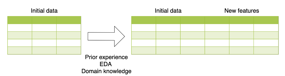
Feature Engineering
You will now get exposure to different types of features. You will modify existing features and create new ones. Also, you will treat the missing data accordingly. This is the Summary of lecture "Winning a Kaggle Competition in Python", via datacamp.


import pandas as pd
import numpy as np
import matplotlib.pyplot as plt

plt.style.use('ggplot')
plt.rcParams['figure.figsize'] = (10, 8)
Arithmetical features
To practice creating new features, you will be working with a subsample from the Kaggle competition called "House Prices: Advanced Regression Techniques". The goal of this competition is to predict the price of the house based on its properties. It's a regression problem with Root Mean Squared Error as an evaluation metric.
Your goal is to create new features and determine whether they improve your validation score. To get the validation score from 5-fold cross-validation, you're given the get_kfold_rmse() function.
from sklearn.ensemble import RandomForestRegressor
from sklearn.model_selection import KFold
from sklearn.metrics import mean_squared_error

kf = KFold(n_splits=5, shuffle=True, random_state=123)

def get_kfold_rmse(train):
    mse_scores = []

    for train_index, test_index in kf.split(train):
        train = train.fillna(0)
        feats = [x for x in train.columns if x not in ['Id', 'SalePrice', 'RoofStyle', 'CentralAir']]

        fold_train, fold_test = train.loc[train_index], train.loc[test_index]

        # Fit the data and make predictions
        # Create a Random Forest object
        rf = RandomForestRegressor(n_estimators=10, min_samples_split=10, random_state=123)

        # Train a model
        rf.fit(X=fold_train[feats], y=fold_train['SalePrice'])

        # Get predictions for the test set
        pred = rf.predict(fold_test[feats])

        fold_score = mean_squared_error(fold_test['SalePrice'], pred)
        mse_scores.append(np.sqrt(fold_score))

    return round(np.mean(mse_scores) + np.std(mse_scores), 2)
train = pd.read_csv('./dataset/house_prices_train.csv')
test = pd.read_csv('./dataset/house_prices_test.csv')
print('RMSE before feature engineering:', get_kfold_rmse(train))

# Find the total area of the house
train['totalArea'] = train['TotalBsmtSF'] + train['1stFlrSF'] + train['2ndFlrSF']

# Look at the updated RMSE
print('RMSE with total area:', get_kfold_rmse(train))

# Find the area of the garden
train['GardenArea'] = train['LotArea'] - train['1stFlrSF']
print('RMSE with garden area:', get_kfold_rmse(train))

# Find total number of bathrooms
train['TotalBath'] = train['FullBath'] + train['HalfBath']
print('RMSE with number of bathromms:', get_kfold_rmse(train))
You've created three new features. Here you see that house area improved the RMSE by almost $1,000. Adding garden area improved the RMSE by another $600. However, with the total number of bathrooms, the RMSE has increased. It means that you keep the new area features, but do not add "TotalBath" as a new feature.
Date features
You've built some basic features using numerical variables. Now, it's time to create features based on date and time. You will practice on a subsample from the Taxi Fare Prediction Kaggle competition data. The data represents information about the taxi rides and the goal is to predict the price for each ride.
Your objective is to generate date features from the pickup datetime. Recall that it's better to create new features for train and test data simultaneously. After the features are created, split the data back into the train and test DataFrames. Here it's done using pandas' isin() method.
train = pd.read_csv('./dataset/taxi_train_chapter_4.csv')
test = pd.read_csv('./dataset/taxi_test_chapter_4.csv')
taxi = pd.concat([train, test])

# Convert pickup date to datetime object
taxi['pickup_datetime'] = pd.to_datetime(taxi['pickup_datetime'])

# Create a day of week feature
taxi['dayofweek'] = taxi['pickup_datetime'].dt.dayofweek

# Create an hour feature
taxi['hour'] = taxi['pickup_datetime'].dt.hour

# Split back into train and test
new_train = taxi[taxi['id'].isin(train['id'])]
new_test = taxi[taxi['id'].isin(test['id'])]
from sklearn.preprocessing import LabelEncoder

train = pd.read_csv('./dataset/house_prices_train.csv')
test = pd.read_csv('./dataset/house_prices_test.csv')

# Concatenate train and test together
houses = pd.concat([train, test])

# Label encoder
le = LabelEncoder()

# Create new features
houses['RoofStyle_enc'] = le.fit_transform(houses['RoofStyle'])
houses['CentralAir_enc'] = le.fit_transform(houses['CentralAir'])

# Look at new features
houses[['RoofStyle', 'RoofStyle_enc', 'CentralAir', 'CentralAir_enc']].head()
One-Hot encoding
The problem with label encoding is that it implicitly assumes that there is a ranking dependency between the categories. So, let's change the encoding method for the features "RoofStyle" and "CentralAir" to one-hot encoding.
Recall that if you're dealing with binary features (categorical features with only two categories) it is suggested to apply label encoder only.
Your goal is to determine which of the mentioned features is not binary, and to apply one-hot encoding only to this one.
houses = pd.concat([train, test])

# Look at feature distributions
print(houses['RoofStyle'].value_counts(), '\n')
print(houses['CentralAir'].value_counts())
le = LabelEncoder()
houses['CentralAir_enc'] = le.fit_transform(houses['CentralAir'])

# Create One-Hot encoded features
ohe = pd.get_dummies(houses['RoofStyle'], prefix='RoofStyle')

# Concatenate OHE features to houses
houses = pd.concat([houses, ohe], axis=1)

# Look at OHE features
houses[[col for col in houses.columns if 'RoofStyle' in col]].head(5)
Mean target encoding
First of all, you will create a function that implements mean target encoding. Remember that you need to develop the two following steps:
- Calculate the mean on the train, apply to the test
- Split train into K folds. Calculate the out-of-fold mean for each fold, apply to this particular fold
def test_mean_target_encoding(train, test, target, categorical, alpha=5):
    # Calculate global mean on the train data
    global_mean = train[target].mean()

    # Group by the categorical feature and calculate its properties
    train_groups = train.groupby(categorical)
    category_sum = train_groups[target].sum()
    category_size = train_groups.size()

    # Calculate smoothed mean target statistics
    train_statistics = (category_sum + global_mean * alpha) / (category_size + alpha)

    # Apply statistics to the test data and fill new categories
    test_feature = test[categorical].map(train_statistics).fillna(global_mean)
    return test_feature.values

def train_mean_target_encoding(train, target, categorical, alpha=5):
    # Create 5-fold cross-validation
    kf = KFold(n_splits=5,random_state=123, shuffle=True)
    train_feature = pd.Series(index=train.index, dtype='float')

    # For each folds split
    for train_index, test_index in kf.split(train):
        cv_train, cv_test = train.iloc[train_index], train.iloc[test_index]

        # Calculate out-of-fold statistics and apply to cv_test
        cv_test_feature = test_mean_target_encoding(cv_train, cv_test, target,
                                                    categorical, alpha)

        # Save new feature for this particular fold
        train_feature.iloc[test_index] = cv_test_feature
    return train_feature.values

def mean_target_encoding(train, test, target, categorical, alpha=5):
    # Get the train feature
    train_feature = train_mean_target_encoding(train, target, categorical, alpha)

    # Get the test feature
    test_feature = test_mean_target_encoding(train, test, target, categorical, alpha)

    # Return new features to add to the model
    return train_feature, test_feature
K-fold cross-validation
You will work with a binary classification problem on a subsample from Kaggle playground competition. The objective of this competition is to predict whether a famous basketball player Kobe Bryant scored a basket or missed a particular shot.
Train data is available in your workspace as bryant_shots DataFrame. It contains data on 10,000 shots with its properties and a target variable "shot\_made\_flag" -- whether shot was scored or not.
One of the features in the data is "game_id" -- a particular game where the shot was made. There are 541 distinct games. So, you deal with a high-cardinality categorical feature. Let's encode it using a target mean!
Suppose you're using 5-fold cross-validation and want to evaluate a mean target encoded feature on the local validation.
bryant_shots = pd.read_csv('./dataset/bryant_shots.csv')

# Create 5-fold cross-validation
kf = KFold(n_splits=5, random_state=123, shuffle=True)

# For each folds split
for train_index, test_index in kf.split(bryant_shots):
    cv_train, cv_test = bryant_shots.iloc[train_index].copy(), bryant_shots.iloc[test_index].copy()

    # Create mean target encoded feature
    cv_train['game_id_enc'], cv_test['game_id_enc'] = mean_target_encoding(train=cv_train,
                                                                           test=cv_test,
                                                                           target='shot_made_flag',
                                                                           categorical='game_id',
                                                                           alpha=5)

    # Look at the encoding
    print(cv_train[['game_id', 'shot_made_flag', 'game_id_enc']].sample(n=1))
You could see different game encodings for each validation split in the output. The main conclusion you should make: while using local cross-validation, you need to repeat mean target encoding procedure inside each folds split separately.
Beyond binary classification
Of course, binary classification is just a single special case. Target encoding could be applied to any target variable type:
- For binary classification usually mean target encoding is used
- For regression mean could be changed to median, quartiles, etc.
- For multi-class classification with N classes we create N features with target mean for each category in one vs. all fashion
The
mean_target_encoding()function you've created could be used for any target type specified above. Let's apply it for the regression problem on the example of House Prices Kaggle competition.
Your goal is to encode a categorical feature "RoofStyle" using mean target encoding.
train = pd.read_csv('./dataset/house_prices_train.csv')
test = pd.read_csv('./dataset/house_prices_test.csv')

# Create mean target encoded feature
train['RoofStyle_enc'], test['RoofStyle_enc'] = mean_target_encoding(train=train,
                                                                     test=test,
                                                                     target='SalePrice',
                                                                     categorical='RoofStyle',
                                                                     alpha=10)
# Look at the encoding
test[['RoofStyle', 'RoofStyle_enc']].drop_duplicates()
You observe that houses with the Hip roof are the most pricy, while houses with the Gambrel roof are the cheapest. It's exactly the goal of target encoding: you've encoded categorical feature in such a manner that there is now a correlation between category values and target variable. We're done with categorical encoders.
Find missing data
Let's impute missing data on a real Kaggle dataset. For this purpose, you will be using a data subsample from the Kaggle "Two sigma connect: rental listing inquiries" competition.
Before proceeding with any imputing you need to know the number of missing values for each of the features. Moreover, if the feature has missing values, you should explore the type of this feature.
twosigma = pd.read_csv('./dataset/twosigma_rental_train_null.csv')

# find the number of missing values in each column
print(twosigma.isnull().sum())

twosigma[['building_id', 'price']].head()
Impute missing data
You've found that "price" and "building_id" columns have missing values in the Rental Listing Inquiries dataset. So, before passing the data to the models you need to impute these values.
Numerical feature "price" will be encoded with a mean value of non-missing prices.
Imputing categorical feature "building_id" with the most frequent category is a bad idea, because it would mean that all the apartments with a missing "building_id" are located in the most popular building. The better idea is to impute it with a new category.
from sklearn.impute import SimpleImputer

# Create mean imputer
mean_imputer = SimpleImputer(strategy='mean')

# Price imputation
twosigma[['price']] = mean_imputer.fit_transform(twosigma[['price']])

# Create constant inputer
constant_imputer = SimpleImputer(strategy='constant', fill_value='MISSING')

# building_id imputation
twosigma[['building_id']] = constant_imputer.fit_transform(twosigma[['building_id']])
twosigma.isnull().sum()