Modeling
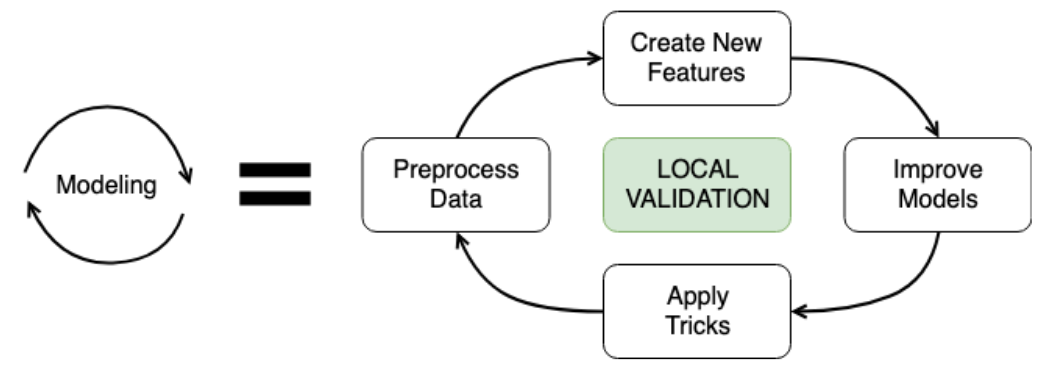
Time to bring everything together and build some models! In this last chapter, you will build a base model before tuning some hyperparameters and improving your results with ensembles. You will then get some final tips and tricks to help you compete more efficiently. This is the Summary of lecture "Winning a Kaggle Competition in Python", via datacamp.


import pandas as pd
import numpy as np
import matplotlib.pyplot as plt

plt.style.use('ggplot')
plt.rcParams['figure.figsize'] = (10, 8)
Replicate validation score
Throughout this chapter, you will work with New York City Taxi competition data. The problem is to predict the fare amount for a taxi ride in New York City. The competition metric is the root mean squared error.
The first goal is to evaluate the Baseline model on the validation data. You will replicate the simplest Baseline based on the mean of "fare_amount". Recall that as a validation strategy we used a 30% holdout split with validation_train as train and validation_test as holdout DataFrames.
from sklearn.model_selection import train_test_split

train = pd.read_csv('./dataset/taxi_train_chapter_4.csv')
test = pd.read_csv('./dataset/taxi_test_chapter_4.csv')

validation_train, validation_test = train_test_split(train, test_size=0.3)
from sklearn.metrics import mean_squared_error
from math import sqrt

# Calculate the mean fare_amount on the validation_train data
naive_prediction = np.mean(validation_train['fare_amount'])

# Assign naive prediction to all the holdout observations
validation_test = validation_test.copy()
validation_test['pred'] = naive_prediction

# Measure the local RMSE
rmse = sqrt(mean_squared_error(validation_test['fare_amount'], validation_test['pred']))
print('Validation RMSE for Baseline I model: {:.3f}'.format(rmse))
Baseline based on the date
We've already built 3 different baseline models. To get more practice, let's build a couple more. The first model is based on the grouping variables. It's clear that the ride fare could depend on the part of the day. For example, prices could be higher during the rush hours.
Your goal is to build a baseline model that will assign the average "fare_amount" for the corresponding hour. For now, you will create the model for the whole train data and make predictions for the test dataset.
train['pickup_datetime'] = pd.to_datetime(train['pickup_datetime'])
test['pickup_datetime'] = pd.to_datetime(test['pickup_datetime'])

# Get pickup hour from the pickup_datetime column
train['hour'] = train['pickup_datetime'].dt.hour
test['hour'] = test['pickup_datetime'].dt.hour

# Calculate average fare_amount grouped by pickup hour
hour_groups = train.groupby('hour')['fare_amount'].mean()

# Make predictions on the test set
test['fare_amount'] = test.hour.map(hour_groups)

# Write predictions
test[['id', 'fare_amount']].to_csv('hour_mean_sub.csv', index=False)
!head hour_mean_sub.csv
Baseline based on the gradient boosting
Let's build a final baseline based on the Random Forest. You've seen a huge score improvement moving from the grouping baseline to the Gradient Boosting in the video. Now, you will use sklearn's Random Forest to further improve this score.
The goal of this exercise is to take numeric features and train a Random Forest model without any tuning. After that, you could make test predictions and validate the result on the Public Leaderboard.
from sklearn.ensemble import RandomForestRegressor

# Select only numeric features
features = ['pickup_longitude', 'pickup_latitude', 'dropoff_longitude',
            'dropoff_latitude', 'passenger_count', 'hour']

# Train a Random Forest model
rf = RandomForestRegressor()
rf.fit(train[features], train.fare_amount)

# Make predictions on the test data
test['fare_amount'] = rf.predict(test[features])

# Write predictions
test[['id', 'fare_amount']].to_csv('rf_sub.csv', index=False)
!head rf_sub.csv
Hyperparameter tuning
- Ridge Regression
- Least squares linear regression $$ \text{Loss} = \sum_{i=1}^N (y_i - \hat{y_i})^2 \rightarrow \text{min} $$
- Ridge Regression $$ \text{Loss} = \sum_{i=1}^N (y_i - \hat{y_i})^2 + \alpha \sum_{j=1}^K w_j^2 \rightarrow \text{min} $$
- $\alpha$ is hyperparameter
- Hyperparameter optimization strategies
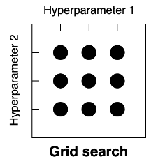
- Grid Search - Choose the predefined grid of hyperparamter values
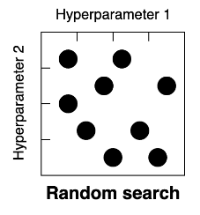
- Random Search - Choose the search space of hyperparamter values
- Bayesian optimization - Choose the search space of hyperparameter values
- Grid Search - Choose the predefined grid of hyperparamter values
Grid search
Recall that we've created a baseline Gradient Boosting model in the previous lesson. Your goal now is to find the best max_depth hyperparameter value for this Gradient Boosting model. This hyperparameter limits the number of nodes in each individual tree. You will be using K-fold cross-validation to measure the local performance of the model for each hyperparameter value.
You're given a function get_cv_score(), which takes the train dataset and dictionary of the model parameters as arguments and returns the overall validation RMSE score over 3-fold cross-validation.
from sklearn.model_selection import KFold
from sklearn.ensemble import GradientBoostingRegressor

def get_cv_score(train, params):
    # Create KFold object
    kf = KFold(n_splits=3, shuffle=True, random_state=123)

    rmse_scores = []

    # Loop through each split
    for train_index, test_index in kf.split(train):
        cv_train, cv_test = train.iloc[train_index], train.iloc[test_index]

        # Train a Gradient Boosting model
        gb = GradientBoostingRegressor(random_state=123, **params).fit(cv_train[features], cv_train.fare_amount)

        # Make predictions on the test data
        pred = gb.predict(cv_test[features])

        fold_score = np.sqrt(mean_squared_error(cv_test['fare_amount'], pred))
        rmse_scores.append(fold_score)

    return np.round(np.mean(rmse_scores) + np.std(rmse_scores), 5)
max_depth_grid = [3, 6, 9, 12, 15]
results = {}

# For each value in the grid
for max_depth_candidate in max_depth_grid:
    # Specify parameters for the model
    params = {'max_depth': max_depth_candidate}

    # Calculate validation score for a particular hyperparameter
    validation_score = get_cv_score(train, params)

    # Save the results for each max depth value
    results[max_depth_candidate] = validation_score
print(results)
2D grid search
The drawback of tuning each hyperparameter independently is a potential dependency between different hyperparameters. The better approach is to try all the possible hyperparameter combinations. However, in such cases, the grid search space is rapidly expanding. For example, if we have 2 parameters with 10 possible values, it will yield 100 experiment runs.
Your goal is to find the best hyperparameter couple of max_depth and subsample for the Gradient Boosting model. subsample is a fraction of observations to be used for fitting the individual trees.
import itertools

# Hyperparameter grids
max_depth_grid = [3, 5, 7]
subsample_grid = [0.8, 0.9, 1.0]
results = {}

# For each couple in the grid
for max_depth_candidate, subsample_candidate in itertools.product(max_depth_grid, subsample_grid):
    params = {'max_depth': max_depth_candidate,
              'subsample': subsample_candidate}
    validation_score = get_cv_score(train, params)
    # Save the results fro each couple
    results[(max_depth_candidate, subsample_candidate)] = validation_score
print(results)
train = pd.read_csv('./dataset/taxi_train_distance.csv')
test = pd.read_csv('./dataset/taxi_test_distance.csv')

features = ['pickup_longitude', 'pickup_latitude', 'dropoff_longitude', 'dropoff_latitude',
            'passenger_count', 'distance_km', 'hour']
gb = GradientBoostingRegressor().fit(train[features], train.fare_amount)

# Train a Random Forest model
rf = RandomForestRegressor().fit(train[features], train.fare_amount)

# Make predictions on the test data
test['gb_pred'] = gb.predict(test[features])
test['rf_pred'] = rf.predict(test[features])

# Find mean of model predictions
test['blend'] = (test['gb_pred'] + test['rf_pred']) / 2
test[['gb_pred', 'rf_pred', 'blend']].head(3)
Model stacking I
Now it's time for stacking. To implement the stacking approach, you will follow the 6 steps:
- Split train data into two parts
- Train multiple models on Part 1
- Make predictions on Part 2
- Make predictions on the test data
- Train a new model on Part 2 using predictions as features
- Make predictions on the test data using the 2nd level model
part_1, part_2 = train_test_split(train, test_size=0.5, random_state=123)

# Train a Gradient Boosting model on Part 1
gb = GradientBoostingRegressor().fit(part_1[features], part_1.fare_amount)

# Train a Random Forest model on Part 1
rf = RandomForestRegressor().fit(part_1[features], part_1.fare_amount)

# Make predictions on the Part 2 data
part_2 = part_2.copy()
part_2['gb_pred'] = gb.predict(part_2[features])
part_2['rf_pred'] = rf.predict(part_2[features])

# Make predictions on the test data
test = test.copy()
test['gb_pred'] = gb.predict(test[features])
test['rf_pred'] = rf.predict(test[features])
Model stacking II
what you've done so far in the stacking implementation:
- Split train data into two parts
- Train multiple models on Part 1
- Make predictions on Part 2
- Make predictions on the test data
Now, your goal is to create a second level model using predictions from steps 3 and 4 as features. So, this model is trained on Part 2 data and then you can make stacking predictions on the test data.
from sklearn.linear_model import LinearRegression

# Create linear regression model without the intercept
lr = LinearRegression(fit_intercept=False)

# Train 2nd level model on the Part 2 data
lr.fit(part_2[['gb_pred', 'rf_pred']], part_2.fare_amount)

# Make stacking predictions on the test data
test['stacking'] = lr.predict(test[['gb_pred', 'rf_pred']])

# Look at the model coefficients
print(lr.coef_)
Usually, the 2nd level model is some simple model like Linear or Logistic Regressions. Also, note that you were not using intercept in the Linear Regression just to combine pure model predictions. Looking at the coefficients, it's clear that 2nd level model has more trust to the Random Forest: 0.7 versus 0.3 for the Gradient Boosting.
Testing Kaggle forum ideas
Unfortunately, not all the Forum posts and Kernels are necessarily useful for your model. So instead of blindly incorporating ideas into your pipeline, you should test them first.
You're given a function get_cv_score(), which takes a train dataset as an argument and returns the overall validation root mean squared error over 3-fold cross-validation.
You should try different suggestions from the Kaggle Forum and check whether they improve your validation score.
def get_cv_score(train):
    features = ['pickup_longitude', 'pickup_latitude',
            'dropoff_longitude', 'dropoff_latitude',
            'passenger_count', 'distance_km', 'hour', 'weird_feature']

    features = [x for x in features if x in train.columns]

    # Create KFold object
    kf = KFold(n_splits=3, shuffle=True, random_state=123)

    rmse_scores = []

    # Loop through each split
    for train_index, test_index in kf.split(train):
        cv_train, cv_test = train.iloc[train_index], train.iloc[test_index]

        # Train a Gradient Boosting model
        gb = GradientBoostingRegressor(random_state=123).fit(cv_train[features], cv_train.fare_amount)

        # Make predictions on the test data
        pred = gb.predict(cv_test[features])

        fold_score = np.sqrt(mean_squared_error(cv_test['fare_amount'], pred))
        rmse_scores.append(fold_score)

    return np.round(np.mean(rmse_scores) + np.std(rmse_scores), 5)
new_train_1 = train.drop('passenger_count', axis=1)

# Compare validation scores
initial_score = get_cv_score(train)
new_score = get_cv_score(new_train_1)

print('Initial score is {} and the new score is {}'.format(initial_score, new_score))
new_train_2 = train.copy()

# Find sum of pickup latitude and ride distance
new_train_2['weird_feature'] = new_train_2['pickup_latitude'] + new_train_2['distance_km']

# Compare validation scores
initial_score = get_cv_score(train)
new_score = get_cv_score(new_train_2)

print('Initial score is {} and the new score is {}'.format(initial_score, new_score))