Decision tree for classification
A Summary of lecture "Machine Learning with Tree-Based Models in Python


import pandas as pd
import numpy as np
import matplotlib.pyplot as plt
import seaborn as sns
Decision tree for classification
- Classification-tree
- Sequence of if-else questions about individual features.
- Objective: infer class labels
- Able to caputre non-linear relationships between features and labels
- Don't require feature scaling(e.g. Standardization)
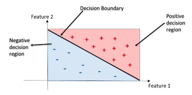
- Decision Regions
- Decision region: region in the feature space where all instances are assigned to one class label
- Decision Boundary: surface separating different decision regions
Train your first classification tree
In this exercise you'll work with the Wisconsin Breast Cancer Dataset from the UCI machine learning repository. You'll predict whether a tumor is malignant or benign based on two features: the mean radius of the tumor (radius_mean) and its mean number of concave points (concave points_mean).
wbc = pd.read_csv('./dataset/wbc.csv')
wbc.head()
X = wbc[['radius_mean', 'concave points_mean']]
y = wbc['diagnosis']
y = y.map({'M':1, 'B':0})
from sklearn.model_selection import train_test_split

X_train, X_test, y_train, y_test = train_test_split(X, y, test_size=0.2, random_state=1)
from sklearn.tree import DecisionTreeClassifier

# Instantiate a DecisionTreeClassifier 'dt' with a maximum depth of 6
dt = DecisionTreeClassifier(max_depth=6, random_state=1)

# Fit dt to the training set
dt.fit(X_train, y_train)

# Predict test set labels
y_pred = dt.predict(X_test)
print(y_pred[0:5])
from sklearn.metrics import accuracy_score

# Predict test set labels
y_pred = dt.predict(X_test)

# Compute test set accuracy
acc = accuracy_score(y_test, y_pred)
print("Test set accuracy: {:.2f}".format(acc))
from mlxtend.plotting import plot_decision_regions

def plot_labeled_decision_regions(X,y, models):
    '''Function producing a scatter plot of the instances contained
    in the 2D dataset (X,y) along with the decision
    regions of two trained classification models contained in the
    list 'models'.

    Parameters
    ----------
    X: pandas DataFrame corresponding to two numerical features
    y: pandas Series corresponding the class labels
    models: list containing two trained classifiers

    '''
    if len(models) != 2:
        raise Exception('''Models should be a list containing only two trained classifiers.''')
    if not isinstance(X, pd.DataFrame):
        raise Exception('''X has to be a pandas DataFrame with two numerical features.''')
    if not isinstance(y, pd.Series):
        raise Exception('''y has to be a pandas Series corresponding to the labels.''')
    fig, ax = plt.subplots(1, 2, figsize=(10.0, 5), sharey=True)
    for i, model in enumerate(models):
        plot_decision_regions(X.values, y.values, model, legend= 2, ax = ax[i])
        ax[i].set_title(model.__class__.__name__)
        ax[i].set_xlabel(X.columns[0])
        if i == 0:
            ax[i].set_ylabel(X.columns[1])
            ax[i].set_ylim(X.values[:,1].min(), X.values[:,1].max())
            ax[i].set_xlim(X.values[:,0].min(), X.values[:,0].max())
    plt.tight_layout()
from sklearn.linear_model import LogisticRegression

# Instantiate logreg
logreg = LogisticRegression(random_state=1)

# Fit logreg to the training set
logreg.fit(X_train, y_train)

# Define a list called clfs containing the two classifiers logreg and dt
clfs = [logreg, dt]

# Review the decision regions of the two classifier
plot_labeled_decision_regions(X_test, y_test, clfs)

Classification tree Learning
- Building Blocks of a Decision-Tree
- Decision-Tree: data structure consisting of a hierarchy of nodes
- Node: question or prediction
- Three kinds of nodes
- Root: no parent node, question giving rise to two children nodes.
- Internal node: one parent node, question giving rise to two children nodes.
- Leaf: one parent node, no children nodes --> prediction.
- Information Gain (IG)
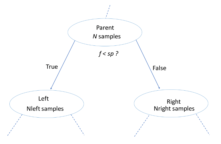 $$ IG(\underbrace{f}_{\text{feature}}, \underbrace{sp}_{\text{split-point}} ) = I(\text{parent}) - \big( \frac{N_{\text{left}}}{N}I(\text{left}) + \frac{N_{\text{right}}}{N}I(\text{right}) \big) $$
- Criteria to measure the impurity of a note $I(\text{node})$:
- gini index
- entropy
- etc...
- Criteria to measure the impurity of a note $I(\text{node})$:
- Classification-Tree Learning
- Nodes are grown recursively.
- At each node, split the data based on:
- feature $f$ and split-point $sp$ to maximize $IG(\text{node})$.
- If $IG(\text{node}) = 0$, declare the node a leaf
from sklearn.tree import DecisionTreeClassifier

# Instantiate dt_entropy, set 'entropy' as the information criterion
dt_entropy = DecisionTreeClassifier(max_depth=8, criterion='entropy', random_state=1)

# Fit dt_entropy to the training set
dt_entropy.fit(X_train, y_train)
Entropy vs Gini index
In this exercise you'll compare the test set accuracy of dt_entropy to the accuracy of another tree named dt_gini. The tree dt_gini was trained on the same dataset using the same parameters except for the information criterion which was set to the gini index using the keyword 'gini'.
dt_gini = DecisionTreeClassifier(max_depth=8, criterion='gini', random_state=1)
dt_gini.fit(X_train, y_train)
from sklearn.metrics import accuracy_score

# Use dt_entropy to predict test set labels
y_pred = dt_entropy.predict(X_test)
y_pred_gini = dt_gini.predict(X_test)

# Evaluate accuracy_entropy
accuracy_entropy = accuracy_score(y_test, y_pred)
accuracy_gini = accuracy_score(y_test, y_pred_gini)

# Print accuracy_entropy
print("Accuracy achieved by using entropy: ", accuracy_entropy)

# Print accuracy_gini
print("Accuracy achieved by using gini: ", accuracy_gini)
Decision tree for regression
- Information Criterion for Regression Tree $$ I(\text{node}) = \underbrace{\text{MSE}(\text{node})}_{\text{mean-squared-error}} = \dfrac{1}{N_{\text{node}}} \sum_{i \in \text{node}} \big(y^{(i)} - \hat{y}_{\text{node}} \big)^2 $$ $$ \underbrace{\hat{y}_{\text{node}}}_{\text{mean-target-value}} = \dfrac{1}{N_{\text{node}}} \sum_{i \in \text{node}}y^{(i)}$$
- Prediction $$ \hat{y}_{\text{pred}}(\text{leaf}) = \dfrac{1}{N_{\text{leaf}}} \sum_{i \in \text{leaf}} y^{(i)}$$
Train your first regression tree
In this exercise, you'll train a regression tree to predict the mpg (miles per gallon) consumption of cars in the auto-mpg dataset using all the six available features.
mpg = pd.read_csv('./dataset/auto.csv')
mpg.head()
mpg = pd.get_dummies(mpg)
mpg.head()
X = mpg.drop('mpg', axis='columns')
y = mpg['mpg']
X_train, X_test, y_train, y_test = train_test_split(X, y, test_size=0.2, random_state=3)
from sklearn.tree import DecisionTreeRegressor

# Instantiate dt
dt = DecisionTreeRegressor(max_depth=8, min_samples_leaf=0.13, random_state=3)

# Fit dt to the training set
dt.fit(X_train, y_train)
Evaluate the regression tree
In this exercise, you will evaluate the test set performance of dt using the Root Mean Squared Error (RMSE) metric. The RMSE of a model measures, on average, how much the model's predictions differ from the actual labels. The RMSE of a model can be obtained by computing the square root of the model's Mean Squared Error (MSE).
from sklearn.metrics import mean_squared_error

# Compute y_pred
y_pred = dt.predict(X_test)

# Compute mse_dt
mse_dt = mean_squared_error(y_test, y_pred)

# Compute rmse_dt
rmse_dt = mse_dt ** (1/2)

# Print rmse_dt
print("Test set RMSE of dt: {:.2f}".format(rmse_dt))
from sklearn.linear_model import LinearRegression

lr = LinearRegression()

lr.fit(X_train, y_train)
y_pred_lr = lr.predict(X_test)

# Compute mse_lr
mse_lr = mean_squared_error(y_test, y_pred_lr)

# Compute rmse_lr
rmse_lr = mse_lr ** 0.5

# Print rmse_lr
print("Linear Regression test set RMSE: {:.2f}".format(rmse_lr))

# Print rmse_dt
print("Regression Tree test set RMSE: {:.2f}".format(rmse_dt))