The Bias-Variance Tradeoff
A Summary of lecture "Machine Learning with Tree-Based Models in Python


import pandas as pd
import numpy as np
import matplotlib.pyplot as plt
import seaborn as sns
Generalization Error
- Supervised Learning - Under the Hood
- supervised learning: $y = f(x)$, $f$ is unknown.
- Goals
- Find a model $\hat{f}$ that best approximates: $f: \hat{f} \approx f$
- $\hat{f}$ can be Logistic Regression, Decision Tree, Neural Network,...
- Discard noise as much as possible
- End goal: $\hat{f}$ should achieve a low predictive error on unseen datasets.
- Difficulties in Approximating $f$
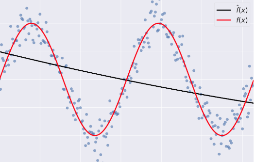
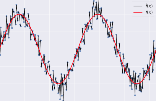
- Overfitting: $\hat{f}(x)$ fits the training set noise.
- Underfitting: $\hat{f}$ is not flexible enough to approximate $f$.
- Generalization Error
- Generalization Error of $\hat{f}$: Does $\hat{f}$ generalize well on unseen data?
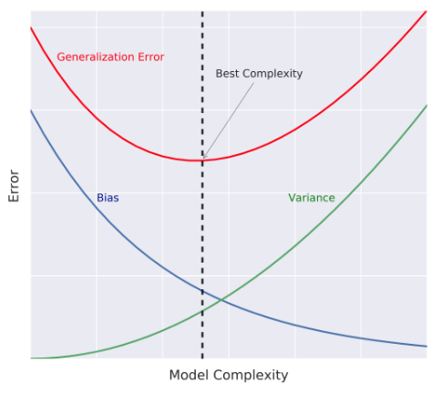
- It can be decomposed as follows: $$ \hat{f} = \text{bias}^2 + \text{variance} +\text{irreducible error} $$
- Bias: error term that tells you, on average, how much $\hat{f} \neq f$.
- Variance: tells you how much $\hat{f}$ is inconsistent over different training sets
- Model Complexity
- Model Complexity: sets the flexibility of $\hat{f}$
- Example: Maximum tree depth, Minimum samples per leaf, ...
- Bias-Variance Tradeoff
Diagnose bias and variance problems
- Estimating the Generalization Error
- How do we estimate the generalization error of a model?
- Cannot be done directly because:
- $f$ is unknown
- usually you only have one dataset
- noise is unpredictable.
- Cannot be done directly because:
- Solution
- Split the data to training and test sets
- fit $\hat{f}$ to the training set
- evaluate the error of $\hat{f}$ on the unseen test set
- generalization error of $\hat{f} \approx$ test set error of $\hat{f}$
- How do we estimate the generalization error of a model?
- Better model Evaluation with Cross-Validation
- Test set should not be touched until we are confident about $\hat{f}$'s performance
- Evaluating $\hat{f}$ on training set: biased estimate, $\hat{f}$ has already seen all training points
- Solution: Cross-Validation (CV)
- K-Fold CV
- Hold-Out CV
- K-Fold CV $$\text{CV error} = \dfrac{E_1 + \cdots + E_{10}}{10} $$
- Diagnose Variance Problems
- If $\hat{f}$ suffers from high variance: CV error of $\hat{f} >$ training set error of $\hat{f}$
- $\hat{f}$ is said to overfit the training set. To remedy overfitting:
- Decrease model complexity
- Gather more data, ...
- $\hat{f}$ is said to overfit the training set. To remedy overfitting:
- If $\hat{f}$ suffers from high variance: CV error of $\hat{f} >$ training set error of $\hat{f}$
- Diagnose Bias Problems
- if $\hat{f}$ suffers from high bias: CV error of $\hat{f} \approx$ training set error of $\hat{f} >>$ desired error.
- $\hat{f}$ is said to underfit the training set. To remedy underfitting:
- Increase model complexity
- Gather more relevant features
mpg = pd.read_csv('./dataset/auto.csv')
mpg.head()
mpg = pd.get_dummies(mpg)
mpg.head()
X = mpg.drop('mpg', axis='columns')
y = mpg['mpg']
from sklearn.model_selection import train_test_split
from sklearn.tree import DecisionTreeRegressor

# Set SEED for reproducibility
SEED = 1

# Split the data into 70% train and 30% test
X_train, X_test, y_train, y_test = train_test_split(X, y, test_size=0.3, random_state=SEED)

# Instantiate a DecisionTreeRegressor dt
dt = DecisionTreeRegressor(max_depth=4, min_samples_leaf=0.26, random_state=SEED)
Evaluate the 10-fold CV error
In this exercise, you'll evaluate the 10-fold CV Root Mean Squared Error (RMSE) achieved by the regression tree dt that you instantiated in the previous exercise.
Note that since cross_val_score has only the option of evaluating the negative MSEs, its output should be multiplied by negative one to obtain the MSEs. The CV RMSE can then be obtained by computing the square root of the average MSE.
from sklearn.model_selection import cross_val_score

# Compute the array containing the 10-folds CV MSEs
MSE_CV_scores = - cross_val_score(dt, X_train, y_train, cv=10,
                                 scoring='neg_mean_squared_error', n_jobs=-1)

# Compute the 10-folds CV RMSE
RMSE_CV = (MSE_CV_scores.mean()) ** 0.5

# Print RMSE_CV
print('CV RMSE: {:.2f}'.format(RMSE_CV))
Evaluate the training error
You'll now evaluate the training set RMSE achieved by the regression tree dt that you instantiated in a previous exercise.
Note that in scikit-learn, the MSE of a model can be computed as follows:
MSE_model = mean_squared_error(y_true, y_predicted)
where we use the function mean_squared_error from the metrics module and pass it the true labels y_true as a first argument, and the predicted labels from the model y_predicted as a second argument.
from sklearn.metrics import mean_squared_error as MSE

# Fit dt to the training set
dt.fit(X_train, y_train)

# Predict the labels of the training set
y_pred_train = dt.predict(X_train)

# Evaluate the training set RMSE of dt
RMSE_train = (MSE(y_train, y_pred_train)) ** 0.5

# Print RMSE_train
print("Train RMSE: {:.2f}".format(RMSE_train))
Ensemble Learning
- Advantages of CARTs
- Simple to understand
- Simple to interpret
- Easy to use
- Flexibility: ability to describe non-linear dependencies.
- Preprocessing: no need to standardize or normalize features.
- Limitations of CARTs
- Classification: can only produce orthogonal decision boundaries
- Sensitive to small variations in the training set
- High variance: unconstrained CARTs may overfit the training set
- Solution: ensemble learning
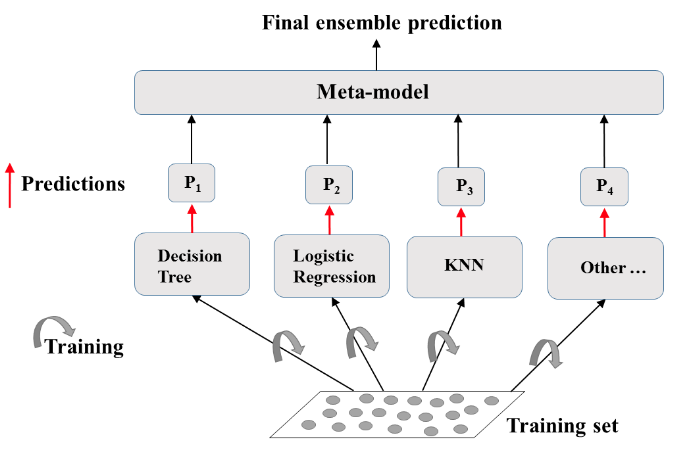
- Ensemble Learning
- Train different models on the same dataset.
- Let each model make its predictions
- Meta-Model: aggregates predictionsof individual models
- Final prediction: more robust and less prone to errors
- Best results: models are skillfull in different ways.
Define the ensemble
In the following set of exercises, you'll work with the Indian Liver Patient Dataset from the UCI Machine learning repository.
In this exercise, you'll instantiate three classifiers to predict whether a patient suffers from a liver disease using all the features present in the dataset.
indian = pd.read_csv('./dataset/indian_liver_patient_preprocessed.csv', index_col=0)
indian.head()
X = indian.drop('Liver_disease', axis='columns')
y = indian['Liver_disease']
X_train, X_test, y_train, y_test = train_test_split(X, y, test_size=0.3, random_state=SEED)
from sklearn.linear_model import LogisticRegression
from sklearn.tree import DecisionTreeClassifier
from sklearn.neighbors import KNeighborsClassifier as KNN

# Set seed for reproducibility
SEED = 1

# Instantiate lr
lr = LogisticRegression(random_state=SEED)

# Instantiate knn
knn = KNN(n_neighbors=27)

# Instantiate dt
dt = DecisionTreeClassifier(min_samples_leaf=0.13, random_state=SEED)

# Define the list classifiers
classifiers = [
    ('Logistic Regression', lr),
    ('K Nearest Neighbors', knn),
    ('Classification Tree', dt)
]
from sklearn.metrics import accuracy_score

# Iterate over the pre-defined list of classifiers
for clf_name, clf in classifiers:
    # Fit clf to the training set
    clf.fit(X_train, y_train)

    # Predict y_pred
    y_pred = clf.predict(X_test)

    # Calculate accuracy
    accuracy = accuracy_score(y_test, y_pred)

    # Evaluate clf's accuracy on the test set
    print('{:s} : {:.3f}'.format(clf_name, accuracy))
from sklearn.ensemble import VotingClassifier

# Instantiate a VotingClassifier vc
vc = VotingClassifier(estimators=classifiers)

# Fit vs to the training set
vc.fit(X_train, y_train)

# Evaluate the test set predictions
y_pred = vc.predict(X_test)

# Calculate accuracy score
accuracy = accuracy_score(y_test, y_pred)
print('Voting Classifier: {:.3f}'.format(accuracy))