Boosting
A Summary of lecture "Machine Learning with Tree-Based Models in Python


import pandas as pd
import numpy as np
import matplotlib.pyplot as plt
import seaborn as sns
Adaboost
- Boosting: Ensemble method combining several weak learners to form a strong learner.
- Weak learner: Model doing slightly better than random guessing
- E.g., Dicision stump (CART whose maximum depth is 1)
- Train an ensemble of predictors sequentially.
- Each predictor tries to correct its predecessor
- Most popular boosting methods:
- AdaBoost
- Gradient Boosting
- Weak learner: Model doing slightly better than random guessing
- AdaBoost
- Stands for Adaptive Boosting
- Each predictor pays more attention to the instances wrongly predicted by its predecessor.
- Achieved by changing the weights of training instances.
- Each predictor is assigned a coefficient $\alpha$ that depends on the predictor's training error
- AdaBoost: Training
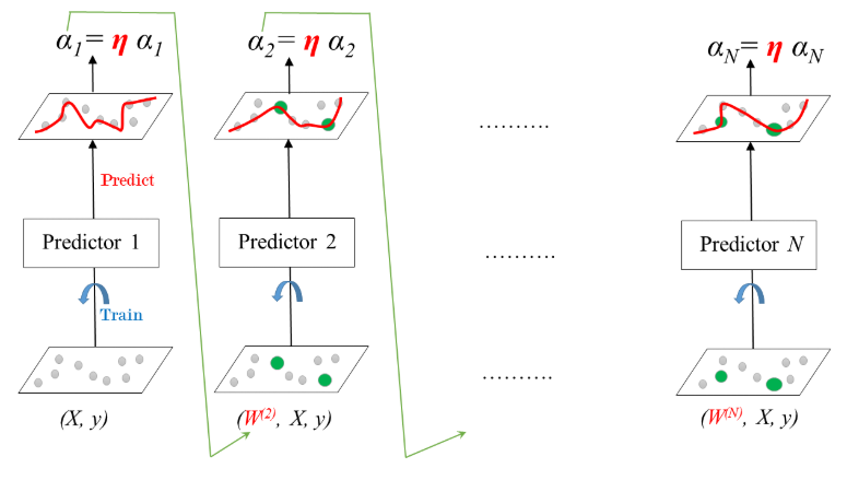
- Learning rate: $0 < \eta < 1$
Define the AdaBoost classifier
In the following exercises you'll revisit the Indian Liver Patient dataset which was introduced in a previous chapter. Your task is to predict whether a patient suffers from a liver disease using 10 features including Albumin, age and gender. However, this time, you'll be training an AdaBoost ensemble to perform the classification task. In addition, given that this dataset is imbalanced, you'll be using the ROC AUC score as a metric instead of accuracy.
As a first step, you'll start by instantiating an AdaBoost classifier.
- Preprocess
indian = pd.read_csv('./datasets/indian_liver_patient_preprocessed.csv', index_col=0)
indian.head()
X = indian.drop('Liver_disease', axis='columns')
y = indian['Liver_disease']
from sklearn.model_selection import train_test_split

X_train, X_test, y_train, y_test = train_test_split(X, y, test_size=0.2, random_state=1)
from sklearn.tree import DecisionTreeClassifier
from sklearn.ensemble import AdaBoostClassifier

# Instantiate dt
dt = DecisionTreeClassifier(max_depth=2, random_state=1)

# Instantiate ada
ada = AdaBoostClassifier(base_estimator=dt, n_estimators=180, random_state=1)
Train the AdaBoost classifier
Now that you've instantiated the AdaBoost classifier ada, it's time train it. You will also predict the probabilities of obtaining the positive class in the test set. This can be done as follows:
Once the classifier ada is trained, call the .predict_proba() method by passing X_test as a parameter and extract these probabilities by slicing all the values in the second column as follows:
ada.predict_proba(X_test)[:,1]
ada.fit(X_train, y_train)

# Compute the probabilities of obtaining the positive class
y_pred_proba = ada.predict_proba(X_test)[:, 1]
Evaluate the AdaBoost classifier
Now that you're done training ada and predicting the probabilities of obtaining the positive class in the test set, it's time to evaluate ada's ROC AUC score. Recall that the ROC AUC score of a binary classifier can be determined using the roc_auc_score() function from sklearn.metrics.
from sklearn.metrics import roc_auc_score

# Evaluate test-set roc_auc_score
ada_roc_auc = roc_auc_score(y_test, y_pred_proba)

# Print roc_auc_score
print('ROC AUC score: {:.2f}'.format(ada_roc_auc))
Gradient Boosting (GB)
- Gradient Boosted Trees
- Sequential correction of predecessor's errors
- Does not tweak the weights of training instances
- Fit each predictor is trained using its predecessor's residual errors as labels
- Gradient Boosted Trees: a CART is used as a base learner.
- Gradient Boosted Trees for Regression: Training
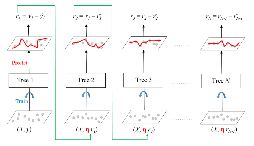
- $\eta$ (shrinkage)
- Ensemble is shrinked after it is multiplied by a learning rate
- $\eta$ (shrinkage)
Define the GB regressor
You'll now revisit the Bike Sharing Demand dataset that was introduced in the previous chapter. Recall that your task is to predict the bike rental demand using historical weather data from the Capital Bikeshare program in Washington, D.C.. For this purpose, you'll be using a gradient boosting regressor.
As a first step, you'll start by instantiating a gradient boosting regressor which you will train in the next exercise.
- Preprocess
bike = pd.read_csv('./datasets/bikes.csv')
bike.head()
X = bike.drop('cnt', axis='columns')
y = bike['cnt']
X_train, X_test, y_train, y_test = train_test_split(X, y, test_size=0.2, random_state=2)
from sklearn.ensemble import GradientBoostingRegressor

# Instantiate gb
gb = GradientBoostingRegressor(max_depth=4, n_estimators=200, random_state=2)
gb.fit(X_train, y_train)

# Predict test set labels
y_pred = gb.predict(X_test)
from sklearn.metrics import mean_squared_error as MSE

# Compute MSE
mse_test = MSE(y_test, y_pred)

# Compute RMSE
rmse_test = mse_test ** 0.5

# Print RMSE
print("Test set RMSE of gb: {:.3f}".format(rmse_test))
Stochastic Gradient Boosting (SGB)
- Gradient Boosting: Cons & Pros
- GB involves an exhaustive search procedure
- Each CART is trained to find the best split points and features.
- May lead to CARTs using the same split points and maybe the same features.
- Stochastic Gradient Boosting
- Each tree is trained on a random subset of rows of the training data.
- The sampled instances (40%-80% of the training set) are sampled without replacement.
- Features are sampled (without replacement) when choosing split points
- Result: further ensemble diversity.
- Effect: adding further variance to the ensemble of trees.
- Stochastic Gradient Boosting: Training
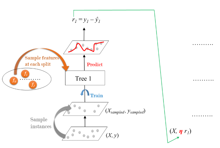
- Residual errors are multiplied by the learning rate $\eta$ and are fed to the next tree in ensemble.
- Process is repeated sequentially until all the trees in the ensemble are trained.
Regression with SGB
As in the exercises from the previous lesson, you'll be working with the Bike Sharing Demand dataset. In the following set of exercises, you'll solve this bike count regression problem using stochastic gradient boosting.
from sklearn.ensemble import GradientBoostingRegressor

# Instantiate sgbr
sgbr = GradientBoostingRegressor(max_depth=4, n_estimators=200, subsample=0.9,
                                 max_features=0.75, random_state=2)
sgbr.fit(X_train, y_train)

# Predict test set labels
y_pred = sgbr.predict(X_test)
from sklearn.metrics import mean_squared_error as MSE

# Compute test set MSE
mse_test = MSE(y_test, y_pred)

# Compute test set RMSE
rmse_test = mse_test ** 0.5

# Print rmse_test
print('Test set RMSE of sgbr: {:.3f}'.format(rmse_test))