K-Means Clustering

• Basics of k-means clustering
  • K-means clustering: first exercise
  • Runtime of k-means clustering
• How many clusters?
  • Elbow method on distinct clusters
  • Elbow method on uniform data
• Limitations of k-means clustering
  • Impact of seeds on distinct clusters
  • Uniform clustering patterns
  • FIFA 18: defenders revisited

import pandas as pd
import numpy as np
import matplotlib.pyplot as plt
import seaborn as sns

Basics of k-means clustering

• Why k-means clustering?
  • A critical drawback of hierarchical clustering: runtime
  • K means runs significantly fater on large datasets
• K-means clustering
  • Generate cluster centers
  • Generate cluster labels

K-means clustering: first exercise

This exercise will familiarize you with the usage of k-means clustering on a dataset. Let us use the Comic Con dataset and check how k-means clustering works on it.

Recall the two steps of k-means clustering:

• Define cluster centers through kmeans() function. It has two required arguments: observations and number of clusters.
• Assign cluster labels through the vq() function. It has two required arguments: observations and cluster centers.

• Preprocess

comic_con = pd.read_csv('./dataset/comic_con.csv', index_col=0)
comic_con.head()

	x_coordinate	y_coordinate
0	17	4
1	20	6
2	35	0
3	14	0
4	37	4

from scipy.cluster.vq import whiten

comic_con['x_scaled'] = whiten(comic_con['x_coordinate'])
comic_con['y_scaled'] = whiten(comic_con['y_coordinate'])

from scipy.cluster.vq import kmeans, vq

# Generate cluster centers
cluster_centers, distortions = kmeans(comic_con[['x_scaled', 'y_scaled']], 2)

# Assign cluster labels
comic_con['cluster_labels'], distortion_list = vq(comic_con[['x_scaled', 'y_scaled']], cluster_centers)

# Plot clusters
sns.scatterplot(x='x_scaled', y='y_scaled', hue='cluster_labels', data=comic_con);

Runtime of k-means clustering

Recall that it took a significantly long time to run hierarchical clustering. How long does it take to run the kmeans() function on the FIFA dataset?

• Preprocess

fifa = pd.read_csv('./dataset/fifa_18_dataset.csv')
fifa.head()

	sliding_tackle	aggression
0	23	63
1	26	48
2	33	56
3	38	78
4	11	29

fifa['scaled_sliding_tackle'] = whiten(fifa['sliding_tackle'])
fifa['scaled_aggression'] = whiten(fifa['aggression'])

from scipy.cluster.hierarchy import linkage

%timeit linkage(fifa[['scaled_sliding_tackle', 'scaled_aggression']], method='ward')

7.19 s ± 10.3 ms per loop (mean ± std. dev. of 7 runs, 1 loop each)

%timeit kmeans(fifa[['scaled_sliding_tackle', 'scaled_aggression']], 2)

69 ms ± 1.21 ms per loop (mean ± std. dev. of 7 runs, 10 loops each)

How many clusters?

• How to find the right k?
  • No absolute method to find right number of clusters(k) in k-means clustering
  • Elbow method
• Distortion
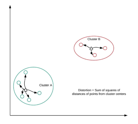
  • sum of squared distances of points from cluster centers
  • Decreases with an increasing number of clusters
  • Becomes zero when the number of clusters equals the numbers of points
  • Elbow plot: line plot between cluster centers and distortion
• Elbow method
  • Elbow plot helps indicate number of clusters present in data
  • Only gives an indication of optimal k
  • Does not always pinpoint how many k
  • Other methods : average silhouette, gap statistic

Elbow method on distinct clusters

Let us use the comic con data set to see how the elbow plot looks on a data set with distinct, well-defined clusters. You may want to display the data points before proceeding with the exercise.

distortions = []
num_clusters = range(1, 7)

# Create a list of distortions from the kmeans function
for i in num_clusters:
    cluster_centers, distortion = kmeans(comic_con[['x_scaled', 'y_scaled']], i)
    distortions.append(distortion)
    
# Create a data frame with two lists - num_clusters, distortions
elbow_plot = pd.DataFrame({'num_clusters': num_clusters, 'distortions': distortions})

# Create a line plot of num_clusters and distortions
sns.lineplot(x='num_clusters', y='distortions', data=elbow_plot);
plt.xticks(num_clusters);

Elbow method on uniform data

In the earlier exercise, you constructed an elbow plot on data with well-defined clusters. Let us now see how the elbow plot looks on a data set with uniformly distributed points. You may want to display the data points on the console before proceeding with the exercise.

• Preprocess

uniform_data = pd.read_csv('./dataset/uniform_data.csv', index_col=0)
uniform_data.head()

	x_coordinate	y_coordinate
0	39	3
1	42	7
2	58	3
3	43	3
4	13	6

uniform_data['x_scaled'] = whiten(uniform_data['x_coordinate'])
uniform_data['y_scaled'] = whiten(uniform_data['y_coordinate'])

distortions = []
num_clusters = range(2, 7)

# Create a list of distortions from the kmeans function
for i in num_clusters:
    cluster_centers, distortion = kmeans(uniform_data[['x_scaled', 'y_scaled']], i)
    distortions.append(distortion)
    
# Create a data frame with two lists - num_clusters, distortions
elbow_plot = pd.DataFrame({'num_clusters': num_clusters, 'distortions': distortions})

# Create a line plot of num_clusters and distortions
sns.lineplot(x='num_clusters', y='distortions', data=elbow_plot);
plt.xticks(num_clusters);

Limitations of k-means clustering

• Limitations of k-means clustering
  • How to find the right K
  • Impact of seeds
  • Biased towards equal sized clusters

Impact of seeds on distinct clusters

You noticed the impact of seeds on a dataset that did not have well-defined groups of clusters. In this exercise, you will explore whether seeds impact the clusters in the Comic Con data, where the clusters are well-defined.

np.random.seed(0)

# Run kmeans clustering
cluster_centers, distortion = kmeans(comic_con[['x_scaled', 'y_scaled']], 2)
comic_con['cluster_labels'], distortion_list = vq(comic_con[['x_scaled', 'y_scaled']], cluster_centers)

# Plot the scatterplot
sns.scatterplot(x='x_scaled', y='y_scaled', hue='cluster_labels', data=comic_con);

np.random.seed([1, 2, 1000])

# Run kmeans clustering
cluster_centers, distortion = kmeans(comic_con[['x_scaled', 'y_scaled']], 2)
comic_con['cluster_labels'], distortion_list = vq(comic_con[['x_scaled', 'y_scaled']], cluster_centers)

# Plot the scatterplot
sns.scatterplot(x='x_scaled', y='y_scaled', hue='cluster_labels', data=comic_con);

Uniform clustering patterns

Now that you are familiar with the impact of seeds, let us look at the bias in k-means clustering towards the formation of uniform clusters.

Let us use a mouse-like dataset for our next exercise. A mouse-like dataset is a group of points that resemble the head of a mouse: it has three clusters of points arranged in circles, one each for the face and two ears of a mouse.

• preprocess

mouse = pd.read_csv('./dataset/mouse.csv', index_col=0)
mouse.head()

	x_coordinate	y_coordinate
0	33.875528	44.893421
1	38.208748	41.116327
2	35.740588	57.418006
3	32.546963	57.218082
4	62.063146	47.196944

mouse['x_scaled'] = whiten(mouse['x_coordinate'])
mouse['y_scaled'] = whiten(mouse['y_coordinate'])

cluster_centers, distortion = kmeans(mouse[['x_scaled', 'y_scaled']], 3)

# Assign cluster labels
mouse['cluster_labels'], distortion_list = vq(mouse[['x_scaled', 'y_scaled']], cluster_centers)

# Plot clusters
sns.scatterplot(x='x_scaled', y='y_scaled', hue='cluster_labels', data=mouse);

FIFA 18: defenders revisited

In the FIFA 18 dataset, various attributes of players are present. Two such attributes are:

• defending: a number which signifies the defending attributes of a player
• physical: a number which signifies the physical attributes of a player

These are typically defense-minded players. In this exercise, you will perform clustering based on these attributes in the data.

• Preprocess

fifa = pd.read_csv('./dataset/fifa_18_sample_data.csv')
fifa.head()

	ID	name	full_name	club	club_logo	special	age	league	birth_date	height_cm	...	prefers_cb	prefers_lb	prefers_lwb	prefers_ls	prefers_lf	prefers_lam	prefers_lcm	prefers_ldm	prefers_lcb	prefers_gk
0	20801	Cristiano Ronaldo	C. Ronaldo dos Santos Aveiro	Real Madrid CF	https://cdn.sofifa.org/18/teams/243.png	2228	32	Spanish Primera División	1985-02-05	185.0	...	False	False	False	False	False	False	False	False	False	False
1	158023	L. Messi	Lionel Messi	FC Barcelona	https://cdn.sofifa.org/18/teams/241.png	2158	30	Spanish Primera División	1987-06-24	170.0	...	False	False	False	False	False	False	False	False	False	False
2	190871	Neymar	Neymar da Silva Santos Jr.	Paris Saint-Germain	https://cdn.sofifa.org/18/teams/73.png	2100	25	French Ligue 1	1992-02-05	175.0	...	False	False	False	False	False	False	False	False	False	False
3	176580	L. Suárez	Luis Suárez	FC Barcelona	https://cdn.sofifa.org/18/teams/241.png	2291	30	Spanish Primera División	1987-01-24	182.0	...	False	False	False	False	False	False	False	False	False	False
4	167495	M. Neuer	Manuel Neuer	FC Bayern Munich	https://cdn.sofifa.org/18/teams/21.png	1493	31	German Bundesliga	1986-03-27	193.0	...	False	False	False	False	False	False	False	False	False	True

5 rows × 185 columns

fifa = fifa[['def', 'phy']].copy()

fifa['scaled_def'] = whiten(fifa['def'])
fifa['scaled_phy'] = whiten(fifa['phy'])

np.random.seed([1000, 2000])

# Fit the data into a k-means algorithm
cluster_centers, _ = kmeans(fifa[['scaled_def', 'scaled_phy']], 3)

# Assign cluster labels
fifa['cluster_labels'], _ = vq(fifa[['scaled_def', 'scaled_phy']], cluster_centers)

# Display cluster centers
print(fifa[['scaled_def', 'scaled_phy', 'cluster_labels']].groupby('cluster_labels').mean())

# Create a scatter plot through seaborn
sns.scatterplot(x='scaled_def', y='scaled_phy', hue='cluster_labels', data=fifa);

                scaled_def  scaled_phy
cluster_labels                        
0                 1.948298    7.163234
1                 3.817844    9.020452
2                 2.072803    9.066327