Feature selection II - selecting for model accuracy
In this second chapter on feature selection, you'll learn how to let models help you find the most important features in a dataset for predicting a particular target feature. In the final lesson of this chapter, you'll combine the advice of multiple, different, models to decide on which features are worth keeping. This is the Summary of lecture "Dimensionality Reduction in Python", via datacamp.


- Selecting features for model performance
- Tree-based feature selection
- Regularized linear regression
- Combining feature selectors
import pandas as pd
import numpy as np
import matplotlib.pyplot as plt
import seaborn as sns

plt.rcParams['figure.figsize'] = (8, 8)
diabetes_df = pd.read_csv('./dataset/PimaIndians.csv')
from sklearn.model_selection import train_test_split
from sklearn.preprocessing import StandardScaler
from sklearn.linear_model import LogisticRegression
from sklearn.metrics import accuracy_score
from pprint import pprint

X, y = diabetes_df.iloc[:, :-1], diabetes_df.iloc[:, -1]
X_train, X_test, y_train, y_test = train_test_split(X, y, test_size=0.3)

scaler = StandardScaler()
lr = LogisticRegression()
X_train_std = scaler.fit_transform(X_train)

# Fit the logistic regression model on the scaled training data
lr.fit(X_train_std, y_train)

# Scaler the test features
X_test_std = scaler.transform(X_test)

# Predict diabetes presence on the scaled test set
y_pred = lr.predict(X_test_std)

# Print accuracy metrics and feature coefficients
print("{0:.1%} accuracy on test set.".format(accuracy_score(y_test, y_pred)))
pprint(dict(zip(X.columns, abs(lr.coef_[0]).round(2))))
We get almost 80% accuracy on the test set. Take a look at the differences in model coefficients for the different features.
X = diabetes_df[['pregnant', 'glucose', 'triceps',
                 'insulin', 'bmi', 'family', 'age']]

# Performs a 25-75% train test split
X_train, X_test, y_train, y_test = train_test_split(X, y, test_size=0.25, random_state=0)

# Scales features and fits the logistic regression model
lr.fit(scaler.fit_transform(X_train), y_train)

# Calculate the accuracy on the test set and prints coefficients
acc = accuracy_score(y_test, lr.predict(scaler.transform(X_test)))
print("{0: .1%} accuracy on test set.".format(acc))
pprint(dict(zip(X.columns, abs(lr.coef_[0]).round(2))))
X = diabetes_df[['glucose', 'triceps', 'bmi', 'family', 'age']]

# Performs a 25-75% train test split
X_train, X_test, y_train, y_test = train_test_split(X, y, test_size=0.25, random_state=0)

# Scales features and fits the logistic regression model
lr.fit(scaler.fit_transform(X_train), y_train)

# Calculates the accuracy on the test set and prints coefficients
acc = accuracy_score(y_test, lr.predict(scaler.transform(X_test)))
print("{0:.1%} accuracy on test set.".format(acc))
pprint(dict(zip(X.columns, abs(lr.coef_[0]).round(2))))
X = diabetes_df[['glucose']]

# Performs a 25-75% train test split
X_train, X_test, y_train, y_test = train_test_split(X, y, test_size=0.25, random_state=0)

# Scales features and fits the logistic regression model to the data
lr.fit(scaler.fit_transform(X_train), y_train)

# Calculates the accuracy on the test set and prints coefficients
acc = accuracy_score(y_test, lr.predict(scaler.transform(X_test)))
print("{0:.1%} accuracy on test set.".format(acc))
print(dict(zip(X.columns, abs(lr.coef_[0]).round(2))))
X, y = diabetes_df.iloc[:, :-1], diabetes_df.iloc[:, -1]
X_train, X_test, y_train, y_test = train_test_split(X, y, test_size=0.3)

lr = LogisticRegression()

# Fit the scaler on the training features and transform these in one go
X_train_std = scaler.fit_transform(X_train)

# Fit the logistic regression model on the scaled training data
lr.fit(X_train_std, y_train)

# Scaler the test features
X_test_std = scaler.transform(X_test)
from sklearn.feature_selection import RFE

# Create the RFE a LogisticRegression estimator and 3 features to select
rfe = RFE(estimator=LogisticRegression(), n_features_to_select=3, verbose=1)

# Fits the eliminator to the data
rfe.fit(X_train_std, y_train)

# Print the features and their ranking (high = dropped early on)
print(dict(zip(X.columns, rfe.ranking_)))

# Print the features that are not elimiated
print(X.columns[rfe.support_])

# CAlculates the test set accuracy
acc = accuracy_score(y_test, rfe.predict(X_test_std))
print("{0:.1%} accuracy on test set.".format(acc))
from sklearn.ensemble import RandomForestClassifier

# Perform a 75% training and 25% test data split
X_train, X_test, y_train, y_test = train_test_split(X, y, test_size=0.25, random_state=0)

# Fit the random forest model to the training data
rf = RandomForestClassifier(random_state=0)
rf.fit(X_train, y_train)

# Calculate the accuracy
acc = accuracy_score(y_test, rf.predict(X_test))

# Print the importances per feature
pprint(dict(zip(X.columns, rf.feature_importances_.round(2))))

# Print accuracy
print("{0:.1%} accuracy on test set.".format(acc))
mask = rf.feature_importances_ > 0.15

# Prints out the mask
print(mask)

# Apply the mask to the feature dataset X
reduced_X = X.loc[:, mask]

# Prints out the selected column names
print(reduced_X.columns)
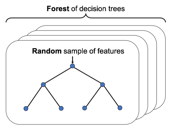
Recursive Feature Elimination with random forests
You'll wrap a Recursive Feature Eliminator around a random forest model to remove features step by step. This method is more conservative compared to selecting features after applying a single importance threshold. Since dropping one feature can influence the relative importances of the others.
rfe = RFE(estimator=RandomForestClassifier(), n_features_to_select=2, verbose=1)

# Fit the model to the training data
rfe.fit(X_train, y_train)

# Create a mask using an attribute of rfe
mask = rfe.support_

# Apply the mask to the feature dataset X and print the result
reduced_X = X.loc[:, mask]
print(reduced_X.columns)
rfe = RFE(estimator=RandomForestClassifier(), n_features_to_select=2, step=2, verbose=1)

# Fit the model to the training data
rfe.fit(X_train, y_train)

# Create a mask using an attribute of rfe
mask = rfe.support_

# Apply the mask to the feature dataset X and print the result
reduced_X = X.loc[:, mask]
print(reduced_X.columns)
Compared to the quick and dirty single threshold method from the previous exercise one of the selected features is different.
Regularized linear regression
- Loss function: Mean Squared Error
- Adding regularization
$$ \text{MSE} + \overbrace{\alpha(\vert \beta_1 \vert + \vert \beta_2 \vert + \vert \beta_3 \vert)}^{\text{Regularization term}} $$
- MSE tries to make model accurate
- Regularization term tries to make model simple
- $\alpha$, when it's too low, the model might overfit. when it's too high, the model might become too simple and inaccurate. One linear model that includes this type of regularization is called Lasso, for Least Absolute Shrinkage and Selection.
Creating a LASSO regressor
You'll be working on the numeric ANSUR body measurements dataset to predict a persons Body Mass Index (BMI) using the Lasso() regressor. BMI is a metric derived from body height and weight but those two features have been removed from the dataset to give the model a challenge.
You'll standardize the data first using the StandardScaler() that has been instantiated for you as scaler to make sure all coefficients face a comparable regularizing force trying to bring them down.
ansur_male = pd.read_csv('./dataset/ANSUR_II_MALE.csv')

ansur_df = ansur_male
# unused columns in the dataset
unused = ['Gender', 'Branch', 'Component', 'BMI_class', 'Height_class', 'weight_kg', 'stature_m']

# Drop the non-numeric columns from df
ansur_df.drop(unused, axis=1, inplace=True)

X = ansur_df.drop('BMI', axis=1)
y = ansur_df['BMI']

scaler = StandardScaler()
from sklearn.linear_model import Lasso

# Set the test size to 30% to get a 70-30% train test split
X_train, X_test, y_train, y_test = train_test_split(X, y, test_size=0.3, random_state=0)

# Fit the scaler on the training features and transform these in one go
X_train_std = scaler.fit_transform(X_train)

# Create the Lasso model
la = Lasso()

# Fit it to the standardized training data
la.fit(X_train_std, y_train)
X_test_std = scaler.transform(X_test)

# Calculate the coefficient of determination (R squared) on X_test_std
r_squared = la.score(X_test_std, y_test)
print("The model can predict {0:.1%} of the variance in the test set.".format(r_squared))

# Create a list that has True values when coefficients equal 0
zero_coef = la.coef_ == 0

# Calculate how many features have a zero coefficient
n_ignored = sum(zero_coef)
print("The model has ignored {} out of {} features.".format(n_ignored, len(la.coef_)))
We can predict almost 85% of the variance in the BMI value using just 9 out of 91 of the features. The $R^2$ could be higher though.
Adjusting the regularization strength
Your current Lasso model has an $R^2$ score of 84.7%. When a model applies overly powerful regularization it can suffer from high bias, hurting its predictive power.
Let's improve the balance between predictive power and model simplicity by tweaking the alpha parameter.
alpha_list = [1, 0.5, 0.1, 0.01]
max_r = 0
max_alpha = 0
for alpha in alpha_list:
    # Find the highest alpha value with R-squared above 98%
    la = Lasso(alpha=alpha, random_state=0)

    # Fits the model and calculates performance stats
    la.fit(X_train_std, y_train)
    r_squared = la.score(X_test_std, y_test)
    n_ignored_features = sum(la.coef_ == 0)

    # Print peformance stats
    print("The model can predict {0:.1%} of the variance in the test set.".format(r_squared))
    print("{} out of {} features were ignored.".format(n_ignored_features, len(la.coef_)))
    if r_squared > 0.98:
        max_r = r_squared
        max_alpha = alpha
        break
print("Max R-squared: {}, alpha: {}".format(max_r, max_alpha))
X = ansur_df[['acromialheight', 'axillaheight', 'bideltoidbreadth', 'buttockcircumference', 'buttockkneelength', 'buttockpopliteallength', 'cervicaleheight', 'chestcircumference', 'chestheight',
       'earprotrusion', 'footbreadthhorizontal', 'forearmcircumferenceflexed', 'handlength', 'headbreadth', 'heelbreadth', 'hipbreadth', 'iliocristaleheight', 'interscyeii',
       'lateralfemoralepicondyleheight', 'lateralmalleolusheight', 'neckcircumferencebase', 'radialestylionlength', 'shouldercircumference', 'shoulderelbowlength', 'sleeveoutseam',
       'thighcircumference', 'thighclearance', 'verticaltrunkcircumferenceusa', 'waistcircumference', 'waistdepth', 'wristheight', 'BMI']]
y = ansur_df['bicepscircumferenceflexed']

X_train, X_test, y_train, y_test = train_test_split(X, y, test_size=0.3, random_state=0)

scaler = StandardScaler()
X_train = scaler.fit_transform(X_train)
X_test = scaler.transform(X_test)
from sklearn.linear_model import LassoCV

# Create and fit the LassoCV model on the training set
lcv = LassoCV()
lcv.fit(X_train, y_train)
print('Optimal alpha = {0:.3f}'.format(lcv.alpha_))

# Calculate R squared on the test set
r_squared = lcv.score(X_test, y_test)
print('The model explains {0:.1%} of the test set variance'.format(r_squared))

# Create a mask for coefficients not equal to zero
lcv_mask = lcv.coef_ != 0
print('{} features out of {} selected'.format(sum(lcv_mask), len(lcv_mask)))
from sklearn.feature_selection import RFE
from sklearn.ensemble import GradientBoostingRegressor

# Select 10 features with RFE on a GradientBoostingRegressor, drop 3 features on each step
rfe_gb = RFE(estimator=GradientBoostingRegressor(),
            n_features_to_select=10, step=3, verbose=1)
rfe_gb.fit(X_train, y_train)

# Calculate the R squared on the test set
r_squared = rfe_gb.score(X_test, y_test)
print('The model can explain {0:.1%} of the variance in the test set'.format(r_squared))

# Assign the support array to gb_mask
gb_mask = rfe_gb.support_
from sklearn.ensemble import RandomForestRegressor

# Select 10 features with RFE on a RandomForestRegressor, drop 3 features on each step
rfe_rf = RFE(estimator=RandomForestRegressor(),
            n_features_to_select=10, step=3, verbose=1)
rfe_rf.fit(X_train, y_train)

# Calculate the R squared on the test set
r_squared = rfe_rf.score(X_test, y_test)
print('The model can explain {0:.1%} of the variance in the test set'.format(r_squared))

# Assign the support array to rf_mask
rf_mask = rfe_rf.support_
Inluding the Lasso linear model from the previous exercise, we now have the votes from 3 models on which features are important.
votes = np.sum([lcv_mask, rf_mask, gb_mask], axis=0)
print(votes)

# Create a mask for features selected by all 3 models
meta_mask = votes == 3
print(meta_mask)

# Apply the dimensionality reduction on X
X_reduced = X.loc[:, meta_mask]
print(X_reduced.columns)
from sklearn.linear_model import LinearRegression

lm = LinearRegression()

# Plug the reduced data into a linear regression pipeline
X_train, X_test, y_train, y_test = train_test_split(X_reduced, y, test_size=0.3, random_state=0)
lm.fit(scaler.fit_transform(X_train), y_train)
r_squared = lm.score(scaler.transform(X_test), y_test)
print('The model can explain {0:.1%} of the variance in the test set using {1:} features.'.format(r_squared, len(lm.coef_)))
Using the votes from 3 models you were able to select just 7 features that allowed a simple linear model to get a high accuracy!