Feature extraction
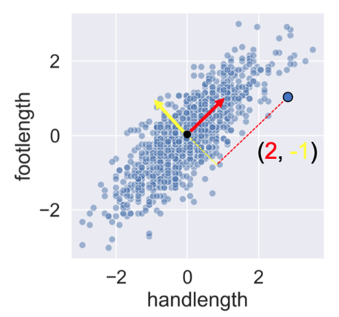
This chapter is a deep-dive on the most frequently used dimensionality reduction algorithm, Principal Component Analysis (PCA). You'll build intuition on how and why this algorithm is so powerful and will apply it both for data exploration and data pre-processing in a modeling pipeline. You'll end with a cool image compression use case. This is the Summary of lecture "Dimensionality Reduction in Python", via datacamp.


import pandas as pd
import numpy as np
import matplotlib.pyplot as plt
import seaborn as sns

plt.rcParams['figure.figsize'] = (8, 8)
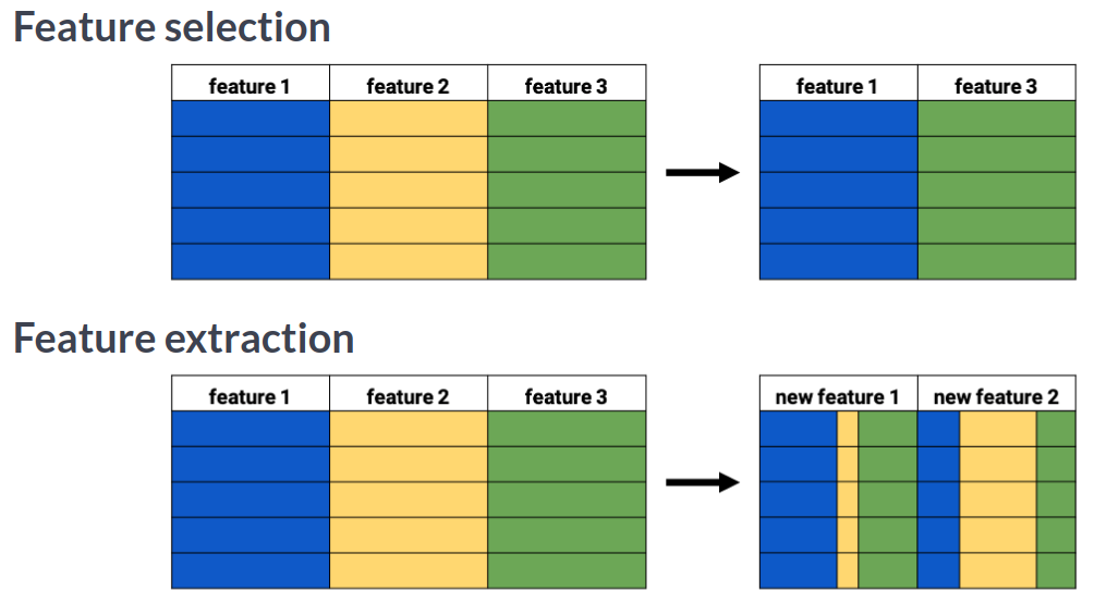
Manual feature extraction I
You want to compare prices for specific products between stores. The features in the pre-loaded dataset sales_df are: storeID, product, quantity and revenue. The quantity and revenue features tell you how many items of a particular product were sold in a store and what the total revenue was. For the purpose of your analysis it's more interesting to know the average price per product.
sales_df = pd.read_csv('./dataset/grocery_sales.csv')
sales_df.head()
sales_df['price'] = sales_df['revenue'] / sales_df['quantity']

# Drop the quantity and revenue features
reduced_df = sales_df.drop(['revenue', 'quantity'], axis=1)

reduced_df.head()
height_df = pd.read_csv('./dataset/height_df.csv')
height_df.head()
height_df['height'] = height_df[['height_1', 'height_2', 'height_3']].mean(axis=1)

# Drop the 3 original height features
reduced_df = height_df.drop(['height_1', 'height_2', 'height_3'], axis=1)

reduced_df.head()
ansur_df = pd.read_csv('./dataset/ansur_sample.csv')
sns.pairplot(ansur_df);

from sklearn.preprocessing import StandardScaler
from sklearn.decomposition import PCA

# Create the scaler and standardize the data
scaler = StandardScaler()
ansur_std = scaler.fit_transform(ansur_df)

# Create the PCA instance and fit and transform the data with pca
pca = PCA()
pc = pca.fit_transform(ansur_std)

# This changes the numpy array output back to a dataframe
pc_df = pd.DataFrame(pc, columns=['PC 1', 'PC 2', 'PC 3', 'PC 4'])

# Create a pairplot of the pricipal component dataframe
sns.pairplot(pc_df);

Notice how, in contrast to the input features, none of the principal components are correlated to one another.
PCA on a larger dataset
You'll now apply PCA on a somewhat larger ANSUR datasample with 13 dimensions. The fitted model will be used in the next exercise. Since we are not using the principal components themselves there is no need to transform the data, instead, it is sufficient to fit pca to the data.
df = pd.read_csv('./dataset/ANSUR_II_MALE.csv')
ansur_df = df[['stature_m', 'buttockheight', 'waistdepth', 'span',
               'waistcircumference', 'shouldercircumference', 'footlength',
               'handlength', 'functionalleglength', 'chestheight',
               'chestcircumference', 'cervicaleheight', 'sittingheight']]
scaler = StandardScaler()
ansur_std = scaler.fit_transform(ansur_df)

# Apply PCA
pca = PCA()
pca.fit(ansur_std)
You've fitted PCA on our 13 feature datasample. Now let's see how the components explain the variance.
print(pca.explained_variance_ratio_)
print(pca.explained_variance_ratio_.cumsum())
Based on the data, we can use 4 principal components if we don't want to lose more than 10% of explained variance during dimensionality reduction.
df = pd.read_csv('./dataset/pokemon.csv')
df.head()
poke_df = df[['HP', 'Attack', 'Defense', 'Sp. Atk', 'Sp. Def', 'Speed']]
poke_df.head()
from sklearn.pipeline import Pipeline

# Build the pipeline
pipe = Pipeline([
    ('scaler', StandardScaler()),
    ('reducer', PCA(n_components=2))
])

# Fit it to the dataset and extract the component vectors
pipe.fit(poke_df)
vectors = pipe.steps[1][1].components_.round(2)

# Print feature effects
print('PC 1 effects = ' + str(dict(zip(poke_df.columns, vectors[0]))))
print('PC 2 effects = ' + str(dict(zip(poke_df.columns, vectors[1]))))
In PC1, All features have a similar positive effect. PC 1 can be interpreted as a measure of overall quality (high stats). In contrast, PC2's defense has a strong positive effect on the second component and speed a strong negative one. This component quantifies an agility vs. armor & protection trade-off.
poke_cat_df = df[['Type 1', 'Legendary']]
pipe = Pipeline([
    ('scaler', StandardScaler()),
    ('reducer', PCA(n_components=2))
])

# Fit the pipeline to poke_df and transform the data
pc = pipe.fit_transform(poke_df)

print(pc)
poke_cat_df.loc[:, 'PC 1'] = pc[:, 0]
poke_cat_df.loc[:, 'PC 2'] = pc[:, 1]

poke_cat_df.head()
sns.scatterplot(data=poke_cat_df, x='PC 1', y='PC 2', hue='Type 1');

sns.scatterplot(data=poke_cat_df, x='PC 1', y='PC 2', hue='Legendary');

Looks like the different types are scattered all over the place while the legendary Pokemon always score high for PC 1 meaning they have high stats overall. Their spread along the PC 2 axis tells us they aren't consistently fast and vulnerable or slow and armored.
from sklearn.ensemble import RandomForestClassifier
from sklearn.model_selection import train_test_split

X = poke_df
y = df['Legendary']

X_train, X_test, y_train, y_test = train_test_split(X, y, test_size=0.3, random_state=0)
pipe = Pipeline([
    ('scaler', StandardScaler()),
    ('reducer', PCA(n_components=2)),
    ('classifier', RandomForestClassifier(random_state=0))
])

# Fit the pipeline to the training data
pipe.fit(X_train, y_train)

# Prints the explained variance ratio
print(pipe.steps[1][1].explained_variance_ratio_)

# Score the acuracy on the test set
accuracy = pipe.score(X_test, y_test)

# Prints the model accuracy
print('{0:.1%} test set accuracy'.format(accuracy))
Repeat the process with 3 extracted components.
pipe = Pipeline([
        ('scaler', StandardScaler()),
        ('reducer', PCA(n_components=3)),
        ('classifier', RandomForestClassifier(random_state=0))])

# Fit the pipeline to the training data
pipe.fit(X_train, y_train)

# Score the accuracy on the test set
accuracy = pipe.score(X_test, y_test)

# Prints the explained variance ratio and accuracy
print(pipe.steps[1][1].explained_variance_ratio_)
print('{0:.1%} test set accuracy'.format(accuracy))
pipe = Pipeline([
        ('scaler', StandardScaler()),
        ('reducer', PCA(n_components=4)),
        ('classifier', RandomForestClassifier(random_state=0))])

# Fit the pipeline to the training data
pipe.fit(X_train, y_train)

# Score the accuracy on the test set
accuracy = pipe.score(X_test, y_test)

# Prints the explained variance ratio and accuracy
print(pipe.steps[1][1].explained_variance_ratio_)
print('{0:.1%} test set accuracy'.format(accuracy))
ansur_df = pd.read_csv('./dataset/ANSUR_II_FEMALE.csv')
ansur_df.head()
ansur_df.drop(['Gender', 'Branch', 'Component', 'BMI_class', 'Height_class'],
              axis=1, inplace=True)
ansur_df.shape
pipe = Pipeline([
    ('scaler', StandardScaler()),
    ('reducer', PCA(n_components=0.8))
])

# Fit the pipe to the data
pipe.fit(ansur_df)

print('{} components selected'.format(len(pipe.steps[1][1].components_)))
pipe = Pipeline([
    ('scaler', StandardScaler()),
    ('reducer', PCA(n_components=0.9))
])

# Fit the pipe to the data
pipe.fit(ansur_df)

print('{} components selected'.format(len(pipe.steps[1][1].components_)))
From the result, we need more than 12 components to go from 80% to 90% explained variance.
pipe = Pipeline([
    ('scaler', StandardScaler()),
    ('reducer', PCA(n_components=10))
])

# Fit the pipe to the data
pipe.fit(ansur_df)

# Plot the explained variance ratio
plt.plot(pipe.steps[1][1].explained_variance_ratio_);
plt.xlabel('Principal component index');
plt.ylabel('Explained variance ratio');
plt.title('Elbow plot of Explained variance ratio');
plt.grid(True);

PCA for image compression
You'll reduce the size of 16 images with hand written digits (MNIST dataset) using PCA.
The samples are 28 by 28 pixel gray scale images that have been flattened to arrays with 784 elements each (28 x 28 = 784) and added to the 2D numpy array X_test. Each of the 784 pixels has a value between 0 and 255 and can be regarded as a feature.
A pipeline with a scaler and PCA model to select 78 components has been pre-loaded for you as pipe. This pipeline has already been fitted to the entire MNIST dataset except for the 16 samples in X_test.
def plot_digits(data):
    fig, axes = plt.subplots(4, 4, figsize=(6, 6),
                             subplot_kw={'xticks':[], 'yticks':[]},
                             gridspec_kw=dict(hspace=0.05, wspace=0.05))
    for i, ax in enumerate(axes.flat):
        ax.imshow(data[i].reshape(28, 28),
                  cmap='binary',
                  clim=(0, 300))
from sklearn.datasets import fetch_openml

X, y = X, y = fetch_openml('mnist_784', version=1, return_X_y=True)
X_train, X_test, y_train, y_test = train_test_split(X, y, test_size=0.3)
X_sample = X_test[:1600:100]
pipe = Pipeline([
    ('scaler', StandardScaler()),
    ('reducer', PCA(n_components=78))
])

pipe.fit(X_train)
plot_digits(X_sample)

pc = pipe.transform(X_sample)

# Prints the number of features per dataset
print("X_test has {} features".format(X_sample.shape[1]))
print("pc has {} features".format(pc.shape[1]))
X_rebuilt = pipe.inverse_transform(pc)

# Prints the number of features
print("X_rebuilt has {} features".format(X_rebuilt.shape[1]))
plot_digits(X_rebuilt)

You've reduced the size of the data 10 fold but were able to reconstruct images with reasonable quality.