Conforming to Statistical Assumptions
In this chapter, you will focus on analyzing the underlying distribution of your data and whether it will impact your machine learning pipeline. You will learn how to deal with skewed data and situations where outliers may be negatively impacting your analysis. This is the Summary of lecture "Feature Engineering for Machine Learning in Python", via datacamp.


import pandas as pd
import numpy as np
import matplotlib.pyplot as plt
import seaborn as sns

plt.rcParams['figure.figsize'] = (8, 8)
What does your data look like? (I)
Up until now you have focused on creating new features and dealing with issues in your data. Feature engineering can also be used to make the most out of the data that you already have and use it more effectively when creating machine learning models.
Many algorithms may assume that your data is normally distributed, or at least that all your columns are on the same scale. This will often not be the case, e.g. one feature may be measured in thousands of dollars while another would be number of years. In this exercise, you will create plots to examine the distributions of some numeric columns in the so_survey_df DataFrame, stored in so_numeric_df.
so_survey_df = pd.read_csv('./dataset/Combined_DS_v10.csv')
so_survey_df.head()
so_numeric_df = so_survey_df[['ConvertedSalary', 'Age', 'Years Experience']]
so_numeric_df.hist();

so_numeric_df[['Age', 'Years Experience']].boxplot();

so_numeric_df[['ConvertedSalary']].boxplot();

sns.pairplot(so_numeric_df);

print(so_numeric_df.describe())
Normalization
As discussed in the video, in normalization you linearly scale the entire column between 0 and 1, with 0 corresponding with the lowest value in the column, and 1 with the largest.
When using scikit-learn (the most commonly used machine learning library in Python) you can use a MinMaxScaler to apply normalization. (It is called this as it scales your values between a minimum and maximum value.)
from sklearn.preprocessing import MinMaxScaler

# Instantiate MinMaxScaler
MM_scaler = MinMaxScaler()

# Fit MM_scaler to the data
MM_scaler.fit(so_numeric_df[['Age']])

# Transform the data using the fitted scaler
so_numeric_df['Age_MM'] = MM_scaler.transform(so_numeric_df[['Age']])

# Compare the original and transformed column
so_numeric_df[['Age_MM', 'Age']].head()
Standardization
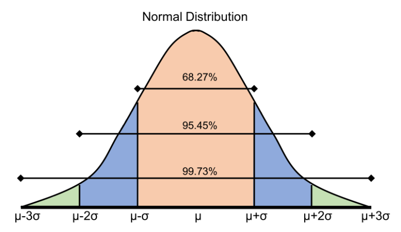
While normalization can be useful for scaling a column between two data points, it is hard to compare two scaled columns if even one of them is overly affected by outliers. One commonly used solution to this is called standardization, where instead of having a strict upper and lower bound, you center the data around its mean, and calculate the number of standard deviations away from mean each data point is.
from sklearn.preprocessing import StandardScaler

# Instantiate StandardScaler
SS_scaler = StandardScaler()

# Fit SS_scaler to the data
SS_scaler.fit(so_numeric_df[['Age']])

# Transform the data using the fitted scaler
so_numeric_df['Age_SS'] = SS_scaler.transform(so_numeric_df[['Age']])

# Compare the original and transformed column
so_numeric_df[['Age_SS', 'Age']].head()
Log transformation
In the previous exercises you scaled the data linearly, which will not affect the data's shape. This works great if your data is normally distributed (or closely normally distributed), an assumption that a lot of machine learning models make. Sometimes you will work with data that closely conforms to normality, e.g the height or weight of a population. On the other hand, many variables in the real world do not follow this pattern e.g, wages or age of a population. In this exercise you will use a log transform on the ConvertedSalary column in the so_numeric_df DataFrame as it has a large amount of its data centered around the lower values, but contains very high values also. These distributions are said to have a long right tail.
from sklearn.preprocessing import PowerTransformer

# Instantiate PowerTransformer
pow_trans = PowerTransformer()

# Train the transform on the data
pow_trans.fit(so_numeric_df[['ConvertedSalary']])

# Apply the power transform to the data
so_numeric_df['ConvertedSalary_LG'] = pow_trans.transform(so_numeric_df[['ConvertedSalary']])

# Plot the data before and after the transformation
so_numeric_df[['ConvertedSalary', 'ConvertedSalary_LG']].hist();

Percentage based outlier removal
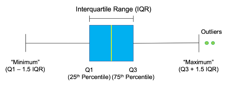
One way to ensure a small portion of data is not having an overly adverse effect is by removing a certain percentage of the largest and/or smallest values in the column. This can be achieved by finding the relevant quantile and trimming the data using it with a mask. This approach is particularly useful if you are concerned that the highest values in your dataset should be avoided. When using this approach, you must remember that even if there are no outliers, this will still remove the same top N percentage from the dataset.
quantile = so_numeric_df['ConvertedSalary'].quantile(0.95)

# Trim the outlier
trimmed_df = so_numeric_df[so_numeric_df['ConvertedSalary'] < quantile]

# The original histogram
so_numeric_df[['ConvertedSalary']].hist();

# The trimmed histogram
trimmed_df[['ConvertedSalary']].hist();


Statistical outlier removal
While removing the top N% of your data is useful for ensuring that very spurious points are removed, it does have the disadvantage of always removing the same proportion of points, even if the data is correct. A commonly used alternative approach is to remove data that sits further than three standard deviations from the mean. You can implement this by first calculating the mean and standard deviation of the relevant column to find upper and lower bounds, and applying these bounds as a mask to the DataFrame. This method ensures that only data that is genuinely different from the rest is removed, and will remove fewer points if the data is close together.
std = so_numeric_df['ConvertedSalary'].std()
mean = so_numeric_df['ConvertedSalary'].mean()

# Calculate the cutoff
cut_off = std * 3
lower, upper = mean - cut_off, mean + cut_off

# Trim the outlier
trimmed_df = so_numeric_df[
    (so_numeric_df['ConvertedSalary'] < upper) &
    (so_numeric_df['ConvertedSalary'] > lower)
]

# Trimmed box plot
trimmed_df[['ConvertedSalary']].boxplot();

Train and testing transformations (I)
So far you have created scalers based on a column, and then applied the scaler to the same data that it was trained on. When creating machine learning models you will generally build your models on historic data (train set) and apply your model to new unseen data (test set). In these cases you will need to ensure that the same scaling is being applied to both the training and test data. To do this in practice you train the scaler on the train set, and keep the trained scaler to apply it to the test set. You should never retrain a scaler on the test set.
from sklearn.model_selection import train_test_split

so_numeric_df = pd.read_csv('./dataset/Combined_DS_v10.csv')[['ConvertedSalary', 'Age', 'Years Experience']]

so_train_numeric, so_test_numeric = train_test_split(so_numeric_df, test_size=0.3)
SS_scaler = StandardScaler()

# Fit the standard scaler to the data
SS_scaler.fit(so_train_numeric[['Age']])

# Transform the test data using the fitted scaler
so_test_numeric['Age_ss'] = SS_scaler.transform(so_test_numeric[['Age']])
so_test_numeric[['Age', 'Age_ss']].head()
Train and testing transformations (II)
Similar to applying the same scaler to both your training and test sets, if you have removed outliers from the train set, you probably want to do the same on the test set as well. Once again you should ensure that you use the thresholds calculated only from the train set to remove outliers from the test set.
train_std = so_train_numeric['ConvertedSalary'].std()
train_mean = so_train_numeric['ConvertedSalary'].mean()

cut_off = train_std * 3
train_lower, train_upper = train_mean - cut_off, train_mean + cut_off

# Trim the test DataFrame
trimmed_df = so_test_numeric[(so_test_numeric['ConvertedSalary'] < train_upper) &
                             (so_test_numeric['ConvertedSalary'] > train_lower)]