TF-IDF and similarity scores
Learn how to compute tf-idf weights and the cosine similarity score between two vectors. You will use these concepts to build a movie and a TED Talk recommender. Finally, you will also learn about word embeddings and using word vector representations, you will compute similarities between various Pink Floyd songs. This is the Summary of lecture "Feature Engineering for NLP in Python", via datacamp.


- Building tf-idf document vectors
- Cosine similarity
- Building a plot line based recommender
- Beyond n-grams: word embeddings
import pandas as pd
import numpy as np
Building tf-idf document vectors
- n-gram modeling
- Weight of dimension dependent on the frequency of the word corresponding to the dimension
- Applications
- Automatically detect stopwords
- Search
- Recommender systems
- Better performance in predictive modeling for some cases
- Term frequency-inverse document frequency
- Proportional to term frequency
- Inverse function of the number of documents in which it occurs
- Mathematical formula
$$ w_{i, j} = \text{tf}_{i, j} \cdot \log (\frac{N}{\text{df}_{i}}) $$
- $w_{i, j} \rightarrow $ weight of term $i$ in document $j$
- $\text{tf}_{i, j} \rightarrow $ term frequency of term $i$ in document $j$
- $N \rightarrow$ number of documents in the corpus
- $\text{df}_{i} \rightarrow$ number of documents containing term $i$
tf-idf vectors for TED talks
In this exercise, you have been given a corpus ted which contains the transcripts of 500 TED Talks. Your task is to generate the tf-idf vectors for these talks.
In a later lesson, we will use these vectors to generate recommendations of similar talks based on the transcript.
df = pd.read_csv('./dataset/ted.csv')
df.head()
ted = df['transcript']
from sklearn.feature_extraction.text import TfidfVectorizer

# Create TfidfVectorizer object
vectorizer = TfidfVectorizer()

# Generate matrix of word vectors
tfidf_matrix = vectorizer.fit_transform(ted)

# Print the shape of tfidf_matrix
print(tfidf_matrix.shape)
You now know how to generate tf-idf vectors for a given corpus of text. You can use these vectors to perform predictive modeling just like we did with CountVectorizer. In the next few lessons, we will see another extremely useful application of the vectorized form of documents: generating recommendations.
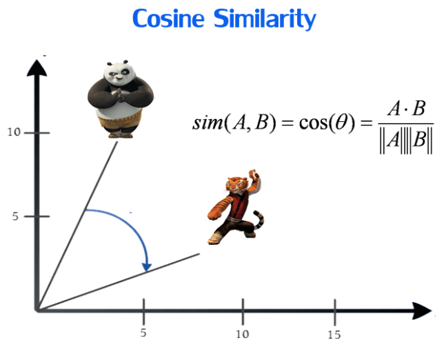
Cosine similarity
-
The dot product
-
Consider two vectors,
$ V = (v_1, v_2, \dots, v_n), W = (w_1, w_2, \dots, w_n) $
-
Then the dot product of $V$ and $W$ is,
$ V \cdot W = (v_1 \times w_1) + (v_2 \times w_2) + \dots + (v_n \times w_n) $
-
-
Magnitude of vector
-
For any vector,
$ V = (v_1, v_2, \dots, v_n) $
-
The magnitude is defined as,
$ \Vert V \Vert = \sqrt{(v_1)^2 + (v_2)^2 + \dots + (v_n)^2} $
-
- Cosine score: points to remember
- Value between -1 and 1
- In NLP, value between 0 (no similarity) and 1 (same)
- Robust to document length
A = np.array([1, 3])
B = np.array([-2, 2])

# Compute dot product
dot_prod = np.dot(A, B)

# Print dot product
print(dot_prod)
Cosine similarity matrix of a corpus
In this exercise, you have been given a corpus, which is a list containing five sentences. You have to compute the cosine similarity matrix which contains the pairwise cosine similarity score for every pair of sentences (vectorized using tf-idf).
Remember, the value corresponding to the ith row and jth column of a similarity matrix denotes the similarity score for the ith and jth vector.
corpus = ['The sun is the largest celestial body in the solar system',
          'The solar system consists of the sun and eight revolving planets',
          'Ra was the Egyptian Sun God',
          'The Pyramids were the pinnacle of Egyptian architecture',
          'The quick brown fox jumps over the lazy dog']
from sklearn.metrics.pairwise import cosine_similarity

# Initialize an instance of tf-idf Vectorizer
tfidf_vectorizer = TfidfVectorizer()

# Generate the tf-idf vectors for the corpus
tfidf_matrix = tfidf_vectorizer.fit_transform(corpus)

# compute and print the cosine similarity matrix
cosine_sim = cosine_similarity(tfidf_matrix, tfidf_matrix)
print(cosine_sim)
As you will see in a subsequent lesson, computing the cosine similarity matrix lies at the heart of many practical systems such as recommenders. From our similarity matrix, we see that the first and the second sentence are the most similar. Also the fifth sentence has, on average, the lowest pairwise cosine scores. This is intuitive as it contains entities that are not present in the other sentences.
Building a plot line based recommender
- Steps
- Text preprocessing
- Generate tf-idf vectors
- Generate cosine-similarity matrix
- The recommender function
- Take a movie title, cosine similarity matrix and indices series as arguments
- Extract pairwise cosine similarity scores for the movie
- Sort the scores in descending order
- Output titles corresponding to the highest scores
- Ignore the highest similarity score (of 1)
Comparing linear_kernel and cosine_similarity
In this exercise, you have been given tfidf_matrix which contains the tf-idf vectors of a thousand documents. Your task is to generate the cosine similarity matrix for these vectors first using cosine_similarity and then, using linear_kernel.
We will then compare the computation times for both functions.
import time

# Record start time
start = time.time()

# Compute cosine similarity matrix
cosine_sim = cosine_similarity(tfidf_matrix, tfidf_matrix)

# Print cosine similarity matrix
print(cosine_sim)

# Print time taken
print("Time taken: %s seconds" % (time.time() - start))
from sklearn.metrics.pairwise import linear_kernel

# Record start time
start = time.time()

# Compute cosine similarity matrix
cosine_sim = linear_kernel(tfidf_matrix, tfidf_matrix)

# Print cosine similarity matrix
print(cosine_sim)

# Print time taken
print("Time taken: %s seconds" % (time.time() - start))
Notice how both linear_kernel and cosine_similarity produced the same result. However, linear_kernel took a smaller amount of time to execute. When you're working with a very large amount of data and your vectors are in the tf-idf representation, it is good practice to default to linear_kernel to improve performance. (NOTE: In case, you see linear_kernel taking more time, it's because the dataset we're dealing with is extremely small and Python's time module is incapable of capture such minute time differences accurately)
The recommender function
In this exercise, we will build a recommender function get_recommendations(), as discussed in the lesson. As we know, it takes in a title, a cosine similarity matrix, and a movie title and index mapping as arguments and outputs a list of 10 titles most similar to the original title (excluding the title itself).
You have been given a dataset metadata that consists of the movie titles and overviews. The head of this dataset has been printed to console.
metadata = pd.read_csv('./dataset/movie_metadata.csv').dropna()
metadata.head()
indices = pd.Series(metadata.index, index=metadata['title']).drop_duplicates()

def get_recommendations(title, cosine_sim, indices):
    # Get the index of the movie that matches the title
    idx = indices[title]
    # Get the pairwsie similarity scores
    sim_scores = list(enumerate(cosine_sim[idx]))
    # Sort the movies based on the similarity scores
    sim_scores = sorted(sim_scores, key=lambda x: x[1], reverse=True)
    # Get the scores for 10 most similar movies
    sim_scores = sim_scores[1:11]
    # Get the movie indices
    movie_indices = [i[0] for i in sim_scores]
    # Return the top 10 most similar movies
    return metadata['title'].iloc[movie_indices]
Plot recommendation engine
In this exercise, we will build a recommendation engine that suggests movies based on similarity of plot lines. You have been given a get_recommendations() function that takes in the title of a movie, a similarity matrix and an indices series as its arguments and outputs a list of most similar movies.
You have also been given a movie_plots Series that contains the plot lines of several movies. Your task is to generate a cosine similarity matrix for the tf-idf vectors of these plots.
Consequently, we will check the potency of our engine by generating recommendations for one of my favorite movies, The Dark Knight Rises.
movie_plots = metadata['overview']
tfidf = TfidfVectorizer(stop_words='english')

# Construct the TF-IDF matrix
tfidf_matrix = tfidf.fit_transform(movie_plots)

# Generate the cosine similarity matrix
cosine_sim = linear_kernel(tfidf_matrix, tfidf_matrix)

# Generate recommendations
print(get_recommendations("The Dark Knight Rises", cosine_sim, indices))
You've just built your very first recommendation system. Notice how the recommender correctly identifies 'The Dark Knight Rises' as a Batman movie and recommends other Batman movies as a result. This sytem is, of course, very primitive and there are a host of ways in which it could be improved. One method would be to look at the cast, crew and genre in addition to the plot to generate recommendations.
TED talk recommender
n this exercise, we will build a recommendation system that suggests TED Talks based on their transcripts. You have been given a get_recommendations() function that takes in the title of a talk, a similarity matrix and an indices series as its arguments, and outputs a list of most similar talks.
You have also been given a transcripts series that contains the transcripts of around 500 TED talks. Your task is to generate a cosine similarity matrix for the tf-idf vectors of the talk transcripts.
Consequently, we will generate recommendations for a talk titled '5 ways to kill your dreams' by Brazilian entrepreneur Bel Pesce.
ted = pd.read_csv('./dataset/ted_clean.csv', index_col=0)
ted.head()
def get_recommendations(title, cosine_sim, indices):
    # Get the index of the movie that matches the title
    idx = indices[title]
    # Get the pairwsie similarity scores
    sim_scores = list(enumerate(cosine_sim[idx]))
    # Sort the movies based on the similarity scores
    sim_scores = sorted(sim_scores, key=lambda x: x[1], reverse=True)
    # Get the scores for 10 most similar movies
    sim_scores = sim_scores[1:11]
    # Get the movie indices
    talk_indices = [i[0] for i in sim_scores]
    # Return the top 10 most similar movies
    return ted['title'].iloc[talk_indices]
indices = pd.Series(ted.index, index=ted['title']).drop_duplicates()
transcripts = ted['transcript']
tfidf = TfidfVectorizer(stop_words='english')

# Construct the TF-IDF matrix
tfidf_matrix = tfidf.fit_transform(transcripts)

# Generate the cosine similarity matrix
cosine_sim = linear_kernel(tfidf_matrix, tfidf_matrix)

# Generate recommendations
print(get_recommendations('5 ways to kill your dreams', cosine_sim, indices))
You have successfully built a TED talk recommender. This recommender works surprisingly well despite being trained only on a small subset of TED talks. In fact, three of the talks recommended by our system is also recommended by the official TED website as talks to watch next after '5 ways to kill your dreams'!
Beyond n-grams: word embeddings
- Word embeddings
- Mapping words into an n-dimensional vector space
- Produced using deep learning and huge amounts of data
- Discern how similar two words are to each other
- Used to detect synonyms and antonyms
- Captures complex relationships
- Dependent on spacy model; independent of dataset you use
en_core_web_lg model (python -m spacy download en_core_web_lg) refer this page
import spacy
nlp = spacy.load('en_core_web_lg')
sent = 'I like apples and orange'

# Create the doc object
doc = nlp(sent)

# Compute pairwise similarity scores
for token1 in doc:
    for token2 in doc:
        print(token1.text, token2.text, token1.similarity(token2))
Notice how the words 'apples' and 'oranges' have the highest pairwaise similarity score. This is expected as they are both fruits and are more related to each other than any other pair of words.
Computing similarity of Pink Floyd songs
In this final exercise, you have been given lyrics of three songs by the British band Pink Floyd, namely 'High Hopes', 'Hey You' and 'Mother'. The lyrics to these songs are available as hopes, hey and mother respectively.
Your task is to compute the pairwise similarity between mother and hopes, and mother and hey.
with open('./dataset/mother.txt', 'r') as f:
    mother = f.read()

with open('./dataset/hopes.txt', 'r') as f:
    hopes = f.read()

with open('./dataset/hey.txt', 'r') as f:
    hey = f.read()
mother_doc = nlp(mother)
hopes_doc = nlp(hopes)
hey_doc = nlp(hey)

# Print similarity between mother and hopes
print(mother_doc.similarity(hopes_doc))

# Print similarity between mother and hey
print(mother_doc.similarity(hey_doc))
Notice that 'Mother' and 'Hey You' have a similarity score of 0.9 whereas 'Mother' and 'High Hopes' has a score of only 0.6. This is probably because 'Mother' and 'Hey You' were both songs from the same album 'The Wall' and were penned by Roger Waters. On the other hand, 'High Hopes' was a part of the album 'Division Bell' with lyrics by David Gilmour and his wife, Penny Samson. Treat yourself by listening to these songs. They're some of the best!