Artificial Neural Networks in PyTorch
In this second chapter, we delve deeper into Artificial Neural Networks, learning how to train them with real datasets. This is the Summary of lecture "Introduction to Deep Learning with PyTorch", via datacamp.


import torch
import torch.nn as nn
import numpy as np
import pandas as pd
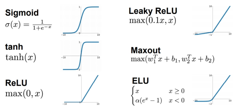
Neural networks
Let us see the differences between neural networks which apply ReLU and those which do not apply ReLU.
We are going to convince ourselves that networks with multiple layers which do not contain non-linearity can be expressed as neural networks with one layer.
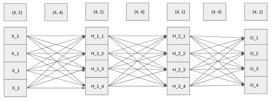
The network and the shape of layers and weights is shown below.
input_layer = torch.tensor([[ 0.0401, -0.9005,  0.0397, -0.0876]])

weight_1 = torch.tensor([[-0.1094, -0.8285,  0.0416, -1.1222],
                        [ 0.3327, -0.0461,  1.4473, -0.8070],
                        [ 0.0681, -0.7058, -1.8017,  0.5857],
                        [ 0.8764,  0.9618, -0.4505,  0.2888]])

weight_2 = torch.tensor([[ 0.6856, -1.7650,  1.6375, -1.5759],
                        [-0.1092, -0.1620,  0.1951, -0.1169],
                        [-0.5120,  1.1997,  0.8483, -0.2476],
                        [-0.3369,  0.5617, -0.6658,  0.2221]])

weight_3 = torch.tensor([[ 0.8824,  0.1268,  1.1951,  1.3061],
                        [-0.8753, -0.3277, -0.1454, -0.0167],
                        [ 0.3582,  0.3254, -1.8509, -1.4205],
                        [ 0.3786,  0.5999, -0.5665, -0.3975]])
hidden_1 = torch.matmul(input_layer, weight_1)
hidden_2 = torch.matmul(hidden_1, weight_2)

# Calculate the output
print(torch.matmul(hidden_2, weight_3))

# Calculate wieght_composed_1 and weight
weight_composed_1 = torch.matmul(weight_1, weight_2)
weight = torch.matmul(weight_composed_1, weight_3)

# Multiply input_layer with weight
print(torch.matmul(input_layer, weight))
relu = nn.ReLU()

# Apply non-linearity on hidden_1 and hidden_2
hidden_1_activated = relu(torch.matmul(input_layer, weight_1))
hidden_2_activated = relu(torch.matmul(hidden_1_activated, weight_2))
print(torch.matmul(hidden_2_activated, weight_3))

# Apply non-linearity in the product of first two weights
weight_composed_1_activated = relu(torch.matmul(weight_1, weight_2))

# Multiply `weight_composed_1_activated` with `weight_3`
weight = torch.matmul(weight_composed_1_activated, weight_3)

# Multiply input_layer with weight
print(torch.matmul(input_layer, weight))
ReLU activation again
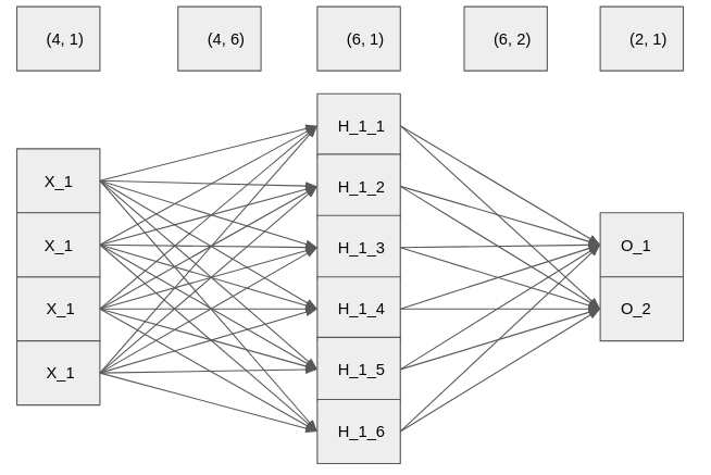
Neural networks don't need to have the same number of units in each layer. Here, you are going to experiment with the ReLU activation function again, but this time we are going to have a different number of units in the layers of the neural network. The input layer will still have 4 features, but then the first hidden layer will have 6 units and the output layer will have 2 units.
weight_1 = torch.rand(4, 6)
weight_2 = torch.rand(6, 2)

# Multiply input_layer with weight_1
hidden_1 = torch.matmul(input_layer, weight_1)

# Apply ReLU activation function over hidden_1 and multiply with weight_2
hidden_1_activated = relu(hidden_1)
print(torch.matmul(hidden_1_activated, weight_2))
Calculating loss function in PyTorch
You are going to code the previous exercise, and make sure that we computed the loss correctly. Predicted scores are -1.2 for class 0 (cat), 0.12 for class 1 (car) and 4.8 for class 2 (frog). The ground truth is class 2 (frog). Compute the loss function in PyTorch.
| Class | Predicted Score |
|---|---|
| Cat | -1.2 |
| Car | 0.12 |
| Frog | 4.8 |
logits = torch.tensor([[-1.2, 0.12, 4.8]])
ground_truth = torch.tensor([2])

# Instantiate cross entropy loss
criterion = nn.CrossEntropyLoss()

# Compute and print the loss
loss = criterion(logits, ground_truth)
print(loss)
the loss function PyTorch calculated gives the same number as the loss function you calculated. Being proficient in understanding and calculating loss functions is a very important skill in deep learning.
logits = torch.rand(1, 1000)
ground_truth = torch.tensor([111])

# Instantiate cross-entropy loss
criterion = nn.CrossEntropyLoss()

# Calculate and print the loss
loss = criterion(logits, ground_truth)
print(loss)
import torchvision
import torchvision.transforms as transforms

# Transform the data to torch tensors and normalize it
transform = transforms.Compose([
    transforms.ToTensor(),
    transforms.Normalize((0.1307), (0.3081))
])

# Preparing training set and test set
trainset = torchvision.datasets.MNIST('mnist', train=True, download=True, transform=transform)
testset = torchvision.datasets.MNIST('mnist', train=False, download=True, transform=transform)

# Prepare training loader and test loader
train_loader = torch.utils.data.DataLoader(trainset, batch_size=32, shuffle=True, num_workers=0)
test_loader = torch.utils.data.DataLoader(testset, batch_size=32, shuffle=False, num_workers=0)
train_data, test_data attributes in dataset is replaced with data
trainset_shape = train_loader.dataset.data.shape
testset_shape = test_loader.dataset.data.shape

# Print the computed shapes
print(trainset_shape, testset_shape)

# Compute the size of the minibatch for training set and test set
trainset_batchsize = train_loader.batch_size
testset_batchsize = test_loader.batch_size

# Print sizes of the minibatch
print(trainset_batchsize, testset_batchsize)
Building a neural network - again
You haven't created a neural network since the end of the first chapter, so this is a good time to build one (practice makes perfect). Build a class for a neural network which will be used to train on the MNIST dataset. The dataset contains images of shape (28, 28, 1), so you should deduct the size of the input layer. For hidden layer use 200 units, while for output layer use 10 units (1 for each class). For activation function, use relu in a functional way.
For context, the same net will be trained and used to make predictions in the next two exercises.
import torch.nn.functional as F

# Define the class Net
class Net(nn.Module):
    def __init__(self):
        # Define all the parameters of the net
        super(Net, self).__init__()
        self.fc1 = nn.Linear(28 * 28 * 1, 200)
        self.fc2 = nn.Linear(200, 10)

    def forward(self, x):
        # Do the forward pass
        x = F.relu(self.fc1(x))
        x = self.fc2(x)
        return x
Training a neural network
Given the fully connected neural network (called model) which you built in the previous exercise and a train loader called train_loader containing the MNIST dataset (which we created for you), you're to train the net in order to predict the classes of digits. You will use the Adam optimizer to optimize the network, and considering that this is a classification problem you are going to use cross entropy as loss function.
import torch.optim as optim

# Instantiate the Adam optimizer and Cross-Entropy loss function
model = Net()
optimizer = optim.Adam(model.parameters(), lr=3e-4)
criterion = nn.CrossEntropyLoss()

for batch_idx, data_target in enumerate(train_loader):
    data = data_target[0]
    target = data_target[1]

    data = data.view(-1, 28 * 28)
    optimizer.zero_grad()

    # Compute a forward pass
    output = model(data)

    # Compute the loss gradients and change the weights
    loss = criterion(output, target)
    loss.backward()
    optimizer.step()
Using the network to make predictions
Now that you have trained the network, use it to make predictions for the data in the testing set. The network is called model (same as in the previous exercise), and the loader is called test_loader. We have already initialized variables total and correct to 0.
correct, total = 0, 0

# Set the model in eval mode
model.eval()

for i, data in enumerate(test_loader, 0):
    inputs, labels = data

    # Put each image into a vector
    inputs = inputs.view(-1, 28 * 28)

    # Do the forward pass and get the predictions
    outputs = model(inputs)
    _, outputs = torch.max(outputs.data, 1)
    total += labels.size(0)
    correct += (outputs == labels).sum().item()
print('The test set accuracy of the network is: %d %%' % (100 * correct / total))