Probability and data generation process
This chapter provides a basic introduction to probability concepts and a hands-on understanding of the data generating process. We'll look at a number of examples of modeling the data generating process and will conclude with modeling an eCommerce advertising simulation. This is the Summary of lecture "Statistical Simulation in Python", via datacamp.


import pandas as pd
import numpy as np
import matplotlib.pyplot as plt
import seaborn as sns

plt.rcParams['figure.figsize'] = (10, 5)
Probability basics
- Probability
- Sample space $S$: Set of all possible outcomes
- Probability $P(A)$: Likelihood of event $A$
- $0\leq P(A) \leq 1$
- $P(S) = 1$ e.g., $P(H) + P(T) = 1$
- For mutually exclusive events $A$ and $B$:
- $P(A \cap B) = 0$
- $P(A \cup B) = P(A) + P(B)$
- Using Simulation for probability Estimation
- Steps for Estimating Probability
- Construct sample space or population
- Determine how to simulate one outcome
- Determine rule for success.
- Sample repeatly and count successes.
- Calculate frequency of successes as an estimate of probability
- Steps for Estimating Probability
Two of a kind
Now let's use simulation to estimate probabilities. Suppose you've been invited to a game of poker at your friend's home. In this variation of the game, you are dealt five cards and the player with the better hand wins. You will use a simulation to estimate the probabilities of getting certain hands. Let's work on estimating the probability of getting at least two of a kind. Two of a kind is when you get two cards of different suites but having the same numeric value (e.g., 2 of hearts, 2 of spades, and 3 other cards).
By the end of this exercise, you will know how to use simulation to calculate probabilities for card games.
np.random.seed(123)

# Shuffle deck & count card occurrences in the hand
n_sims, two_kind = 10000, 0
for i in range(n_sims):
    np.random.shuffle(deck_of_cards)
    hand, cards_in_hand = deck_of_cards[0:5], {}
    for card in hand:
        # Use .get() method on cards_in_hand
        cards_in_hand[card[1]] = cards_in_hand.get(card[1], 0) + 1

    # Condition for getting at least 2 of a kind
    highest_card = max(cards_in_hand.values())
    if highest_card>=2:
        two_kind += 1

print("Probability of seeing at least two of a kind = {} ".format(two_kind/n_sims))
Game of thirteen
A famous French mathematician Pierre Raymond De Montmart, who was known for his work in combinatorics, proposed a simple game called as Game of Thirteen. You have a deck of 13 cards, each numbered from 1 through 13. Shuffle this deck and draw cards one by one. A coincidence is when the number on the card matches the order in which the card is drawn. For instance, if the 5th card you draw happens to be a 5, it's a coincidence. You win the game if you get through all the cards without any coincidences. Let's calculate the probability of winning at this game using simulation.
By completing this exercise, you will further strengthen your ability to cast abstract problems into the simulation framework for estimating probabilities.
np.random.seed(111)

# Pre-set constant variables
deck, sims, coincidences = np.arange(1, 14), 10000, 0

for _ in range(sims):
    # Draw all the cards without replacement to simulate one game
    draw = np.random.choice(deck, size=13, replace=False)
    # Check if there are any coincidences
    coincidence = (draw == list(np.arange(1, 14))).any()
    if coincidence == 0:
        coincidences += 1

# Calculate probability of winning
prob_of_winning = coincidences / sims
print("Probability of winning = {}".format(prob_of_winning))
More probability concepts
- Conditional Probability
- $P(A \vert B) = \frac{P(A \cap B)}{P(B)}$
- $P(B \vert A) = \frac{P(B \cap A)}{P(A)}$
- $P(A \cap B) = P(B \cap A)$
- Bayes Rule
- $P(A \vert B) = \frac{P(B \vert A)P(A)}{P(B)}$
- Independent Events
- $P(A \cap B) = P(A)P(B)$
- $P(A \vert B) = \frac{P(A \cap B)}{P(B)} = \frac{P(A)P(B)}{P(B)} = P(A)$
The conditional urn
As we've learned, conditional probability is defined as the probability of an event given another event. To illustrate this concept, let's turn to an urn problem.
We have an urn that contains 7 white and 6 black balls. Four balls are drawn at random. We'd like to know the probability that the first and third balls are white, while the second and the fourth balls are black.
Upon completion, you will learn to manipulate simulations to calculate simple conditional probabilities.
np.random.seed(123)

# Initialize success, sims and urn
success, sims = 0, 5000
urn = ['w', 'w', 'w', 'w', 'w', 'w', 'w', 'b', 'b', 'b', 'b', 'b', 'b']

for _ in range(sims):
    # Draw 4 balls without replacement
    draw = np.random.choice(urn, replace=False, size=4)
    # Count the number of successes
    if draw[0] == 'w' and draw[1] == 'b' and draw[2] == 'w' and draw[3] == 'b':
        success +=1

print("Probability of success = {}".format(success/sims))
Birthday problem
Now we'll use simulation to solve a famous probability puzzle - the birthday problem. It sounds quite straightforward - How many people do you need in a room to ensure at least a 50% chance that two of them share the same birthday?
With 366 people in a 365-day year, we are 100% sure that at least two have the same birthday, but we only need to be 50% sure. Simulation gives us an elegant way of solving this problem.
Upon completion of this exercise, you will begin to understand how to cast problems in a simulation framework.
np.random.seed(111)

# Draw a sample of birthdays & check if each birthday is unique
days = np.arange(1, 366)
people = 2

def birthday_sim(people):
    sims, unique_birthdays = 2000, 0
    for _ in range(sims):
        draw = np.random.choice(days, size=people, replace=True)
        if len(draw) == len(set(draw)):
            unique_birthdays += 1
    out = 1 - unique_birthdays / sims
    return out

# Break out of the loop if probability greater than 0.5
while (people > 0):
    prop_bds = birthday_sim(people)
    if prop_bds > 0.5:
        break
    people += 1

print("With {} people, there's a 50% chance that two share a birthday.".format(people))
Full house
Let's return to our poker game. Last time, we calculated the probability of getting at least two of a kind. This time we are interested in a full house. A full house is when you get two cards of different suits that share the same numeric value and three other cards that have the same numeric value (e.g., 2 of hearts & spades, jacks of clubs, diamonds, & spades).
Thus, a full house is the probability of getting exactly three of a kind conditional on getting exactly two of a kind of another value. Using the same code as before, modify the success condition to get the desired output. This exercise will teach you to estimate conditional probabilities in card games and build your foundation in framing abstract problems for simulation.
np.random.seed(123)

#Shuffle deck & count card occurrences in the hand
n_sims, full_house, deck_of_cards = 50000, 0, deck.copy()
for i in range(n_sims):
    np.random.shuffle(deck_of_cards)
    hand, cards_in_hand = deck_of_cards[0:5], {}
    for card in hand:
        # Use .get() method to count occurrences of each card
        cards_in_hand[card[1]] = cards_in_hand.get(card[1], 0) + 1

    # Condition for getting full house
    condition = (max(cards_in_hand.values()) ==3) & (min(cards_in_hand.values())==2)
    if  condition == 1:
        full_house += 1
print("Probability of seeing a full house = {}".format(full_house/n_sims))
Driving test
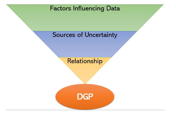
Through the next exercises, we will learn how to build a data generating process (DGP) through progressively complex examples.
In this exercise, you will simulate a very simple DGP. Suppose that you are about to take a driving test tomorrow. Based on your own practice and based on data you have gathered, you know that the probability of you passing the test is 90% when it's sunny and only 30% when it's raining. Your local weather station forecasts that there's a 40% chance of rain tomorrow. Based on this information, you want to know what is the probability of you passing the driving test tomorrow.
This is a simple problem and can be solved analytically. Here, you will learn how to model a simple DGP and see how it can be used for simulation.
np.random.seed(222)
sims, outcomes, p_rain, p_pass = 1000, [], 0.40, {'sun':0.9, 'rain':0.3}

def test_outcome(p_rain):
    # Simulate whether it will rain or not
    weather = np.random.choice(['rain', 'sun'], p=[p_rain, 1 - p_rain])
    # Simulate and return whether you will pass or fail
    return np.random.choice(['pass', 'fail'], p=[p_pass[weather], 1 - p_pass[weather]])

for _ in range(sims):
    outcomes.append(test_outcome(p_rain))

# Calculate fraction of outcomes where you pass
pass_outcomes_frac = np.sum(np.array(outcomes) == 'pass') / len(outcomes)
print("Probability of Passing the driving test = {}".format(pass_outcomes_frac))
National elections
This exercise will give you a taste of how you can model a DGP at different levels of complexity.
Consider national elections in a country with two political parties - Red and Blue. This country has 50 states and the party that wins the most states wins the elections. You have the probability p of Red winning in each individual state and want to know the probability of Red winning nationally.
Let's model the DGP to understand the distribution. Suppose the election outcome in each state follows a binomial distribution with probability p such that 0 indicates a loss for Red and 1 indicates a win. We then simulate a number of election outcomes. Finally, we can ask rich questions like what is the probability of Red winning less than 45% of the states?
p = np.array([0.52076814, 0.67846401, 0.82731745, 0.64722761, 0.03665174,
       0.17835411, 0.75296372, 0.22206157, 0.72778372, 0.28461556,
       0.72545221, 0.106571  , 0.09291364, 0.77535718, 0.51440142,
       0.89604586, 0.39376099, 0.24910244, 0.92518253, 0.08165597,
       0.4212476 , 0.74123879, 0.2479099 , 0.46125805, 0.19584491,
       0.24440482, 0.349916  , 0.80224624, 0.80186664, 0.82968251,
       0.91178779, 0.51739059, 0.67338858, 0.15675863, 0.37772308,
       0.77134621, 0.71727114, 0.92700912, 0.28386132, 0.25502498,
       0.30081506, 0.19724585, 0.29129564, 0.56623386, 0.97681039,
       0.96263926, 0.0548948 , 0.14092758, 0.54739446, 0.54555576])
np.random.seed(224)
outcomes, sims, probs = [], 1000, p

for _ in range(sims):
    # Simulate elections in the 50 states
    election = np.random.binomial(p=probs, n=1)
    # Get average of Red wins and add to `outcomes`
    outcomes.append(np.mean(election))

# Calculate probability of Red winning in less than 45% of the states
prob_red_wins = np.sum(np.array(outcomes) < 0.45) / len(outcomes)
print("Probability of Red winning in less than 45% of the states = {}".format(prob_red_wins))
Fitness goals
Let's model how activity levels impact weight loss using modern fitness trackers. On days when you go to the gym, you average around 15k steps, and around 5k steps otherwise. You go to the gym 40% of the time. Let's model the step counts in a day as a Poisson random variable with a mean $\lambda$ dependent on whether or not you go to the gym.
For simplicity, let’s say you have an 80% chance of losing 1lb and a 20% chance of gaining 1lb when you get more than 10k steps. The probabilities are reversed when you get less than 8k steps. Otherwise, there's an even chance of gaining or losing 1lb. Given all this information, find the probability of losing weight in a month.
np.random.seed(222)
days = 30
# Simulate steps & choose prob
for _ in range(sims):
    w = []
    for i in range(days):
        lam = np.random.choice([5000, 15000], p=[0.6, 0.4], size=1)
        steps = np.random.poisson(lam)
        if steps > 10000:
            prob = [0.2, 0.8]
        elif steps < 8000:
            prob = [0.8, 0.2]
        else:
            prob = [0.5, 0.5]
        w.append(np.random.choice([1, -1], p=prob))
    outcomes.append(sum(w))

# Calculate fraction of outcomes where there was a weight loss
weight_loss_outcomes_frac = np.sum(np.array(outcomes) < 0) / len(outcomes)
print("Probability of Weight Loss = {}".format(weight_loss_outcomes_frac))
Sign up Flow
We will now model the DGP of an eCommerce ad flow starting with sign-ups.
On any day, we get many ad impressions, which can be modeled as Poisson random variables (RV). You are told that λ is normally distributed with a mean of 100k visitors and standard deviation 2000.
During the signup journey, the customer sees an ad, decides whether or not to click, and then whether or not to signup. Thus both clicks and signups are binary, modeled using binomial RVs. What about probability p of success? Our current low-cost option gives us a click-through rate of 1% and a sign-up rate of 20%. A higher cost option could increase the clickthrough and signup rate by up to 20%, but we are unsure of the level of improvement, so we model it as a uniform RV.
np.random.seed(123)

# Initialize click-through rate and signup rate dictionaries
ct_rate = {'low':0.01, 'high':np.random.uniform(low=0.01, high=1.2*0.01)}
su_rate = {'low':0.2, 'high':np.random.uniform(low=0.2, high=1.2*0.2)}

def get_signups(cost, ct_rate, su_rate, sims):
    lam = np.random.normal(loc=100000, scale=2000, size=sims)
    # Simulate impressions(poisson), clicks(binomial) and signups(binomial)
    impressions = np.random.poisson(lam, size=sims)
    clicks = np.random.binomial(n=impressions, p=ct_rate[cost])
    signups = np.random.binomial(n=clicks, p=su_rate[cost])
    return signups

print("Simulated Signups = {}".format(get_signups('high', ct_rate, su_rate, 1)))
Purchase Flow
After signups, let's model the revenue generation process. Once the customer has signed up, they decide whether or not to purchase - a natural candidate for a binomial RV. Let's assume that 10% of signups result in a purchase.
Although customers can make many purchases, let's assume one purchase. The purchase value could be modeled by any continuous RV, but one nice candidate is the exponential RV. Suppose we know that purchase value per customer has averaged around \$1000. We use this information to create the purchase_values RV. The revenue, then, is simply the sum of all purchase values.
def get_signups(cost, ct_rate, su_rate, sims):
    np.random.seed(123)
    lam = np.random.normal(loc=100000, scale=2000, size=sims)
    impressions = np.random.poisson(lam=lam)
    clicks = np.random.binomial(impressions, p=ct_rate[cost])
    signups = np.random.binomial(clicks, p=su_rate[cost])
    return signups
def get_revenue(signups):
    rev = []
    np.random.seed(123)
    for s in signups:
        # Model purchases as binomial, purchase_values as exponential
        purchases = np.random.binomial(s, p=0.1)
        purchase_values = np.random.exponential(scale=1000, size=purchases)

        # Append to revenue the sum of all purchase values.
        rev.append(sum(purchase_values))
    return rev

print("Simulated Revenue = ${}".format(get_revenue(get_signups('low', ct_rate, su_rate, 1))[0]))
Probability of losing money
In this exercise, we will use the DGP model to estimate probability.
As seen earlier, this company has the option of spending extra money, let's say \$3000, to redesign the ad. This could potentially get them higher clickthrough and signup rates, but this is not guaranteed. We would like to know whether or not to spend this extra \\$3000 by calculating the probability of losing money. In other words, the probability that the revenue from the high-cost option minus the revenue from the low-cost option is lesser than the cost.
Once we have simulated revenue outcomes, we can ask a rich set of questions that might not have been accessible using traditional analytical methods.
This simple yet powerful framework forms the basis of Bayesian methods for getting probabilities.
sims, cost_diff = 10000, 3000

# Get revenue when the cost is 'low' and when the cost is 'high'
rev_low = get_revenue(get_signups('low', ct_rate, su_rate, sims))
rev_high = get_revenue(get_signups('high', ct_rate, su_rate, sims))

# calculate fraction of times rev_high - rev_low is less than cost_diff
frac = np.sum((np.array(rev_high) - np.array(rev_low)) < cost_diff) / sims
print("Probability of losing money = {}".format(frac))