Resampling methods
In this chapter, we will get a brief introduction to resampling methods and their applications. We will get a taste of bootstrap resampling, jackknife resampling, and permutation testing. After completing this chapter, students will be able to start applying simple resampling methods for data analysis. This is the Summary of lecture "Statistical Simulation in Python", via datacamp.


- Introduction to resampling method
- Probability example
- Bootstrapping
- Jackknife resampling
- Basic jackknife estimation - mean
- Permutation testing
import pandas as pd
import numpy as np
import matplotlib.pyplot as plt

plt.rcParams['figure.figsize'] = (10, 5)
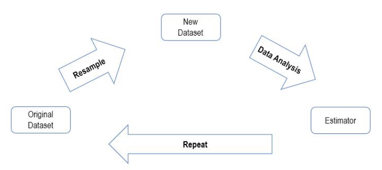
Introduction to resampling method
- Resampling workflow
- Why resample?
- Advantage
- Simple implementation procedure
- Applicable to complex estimators
- No strict assumptions
- Drawbacks
- Computationally expensive
- Advantage
- Types of resampling methods
- Bootstrapping : Sampling with replacement
- Jackknife : Leave out one or more data points (similar to bootstrapping except no random sampling)
- Usefult for estimating bias and variance of estimators
- Permutation testing : Label switching
Probability example
In this exercise, we will review the difference between sampling with and without replacement. We will calculate the probability of an event using simulation, but vary our sampling method to see how it impacts probability.
Consider a bowl filled with colored candies - three blue, two green, and five yellow. Draw three candies at random, with replacement and without replacement. You want to know the probability of drawing a yellow candy on the third draw given that the first candy was blue and the second candy was green.
np.random.seed(123)

# Set up the bowl
success_rep, success_no_rep, sims = 0, 0, 10000
bowl = ['b', 'b', 'b', 'g', 'g', 'y', 'y', 'y', 'y', 'y']

for i in range(sims):
    # Sample with and without replacement & increment success counters
    sample_rep = np.random.choice(bowl, size=3, replace=True)
    sample_no_rep = np.random.choice(bowl, size=3, replace=False)
    if (sample_rep[0] == 'b') & (sample_rep[1] == 'g') & (sample_rep[2] == 'y'):
        success_rep += 1
    if (sample_no_rep[0] == 'b') & (sample_no_rep[1] == 'g') & (sample_no_rep[2] == 'y'):
        success_no_rep += 1

# Calculate probabilities
prob_with_replacement = success_rep / sims
prob_without_replacement = success_no_rep / sims
print("Probability with replacement = {}, without replacement = {}".format(prob_with_replacement,
                                                                           prob_without_replacement))
Running a simple bootstrap
Welcome to the first exercise in the bootstrapping section. We will work through an example where we learn to run a simple bootstrap. As we saw in the video, the main idea behind bootstrapping is sampling with replacement.
Suppose you own a factory that produces wrenches. You want to be able to characterize the average length of the wrenches and ensure that they meet some specifications. Your factory produces thousands of wrenches every day, but it's infeasible to measure the length of each wrench. However, you have access to a representative sample of 100 wrenches. Let's use bootstrapping to get the 95% confidence interval (CI) for the average lengths.
wrench_lengths = np.array([ 8.9143694 , 10.99734545, 10.2829785 ,  8.49370529,  9.42139975,
       11.65143654,  7.57332076,  9.57108737, 11.26593626,  9.1332596 ,
        9.32111385,  9.90529103, 11.49138963,  9.361098  ,  9.55601804,
        9.56564872, 12.20593008, 12.18678609, 11.0040539 , 10.3861864 ,
       10.73736858, 11.49073203,  9.06416613, 11.17582904,  8.74611933,
        9.3622485 , 10.9071052 ,  8.5713193 ,  9.85993128,  9.1382451 ,
        9.74438063,  7.20141089,  8.2284669 ,  9.30012277, 10.92746243,
        9.82636432, 10.00284592, 10.68822271,  9.12046366, 10.28362732,
        9.19463348,  8.27233051,  9.60910021, 10.57380586, 10.33858905,
        9.98816951, 12.39236527, 10.41291216, 10.97873601, 12.23814334,
        8.70591468,  8.96121179, 11.74371223,  9.20193726, 10.02968323,
       11.06931597, 10.89070639, 11.75488618, 11.49564414, 11.06939267,
        9.22729129, 10.79486267, 10.31427199,  8.67373454, 11.41729905,
       10.80723653, 10.04549008,  9.76690794,  8.80169886, 10.19952407,
       10.46843912,  9.16884502, 11.16220405,  8.90279695,  7.87689965,
       11.03972709,  9.59663396,  9.87397041,  9.16248328,  8.39403724,
       11.25523737,  9.31113102, 11.66095249, 10.80730819,  9.68524185,
        8.9140976 ,  9.26753801,  8.78747687, 12.08711336, 10.16444123,
       11.15020554,  8.73264795, 10.18103513, 11.17786194,  9.66498924,
       11.03111446,  8.91543209,  8.63652846, 10.37940061,  9.62082357])
np.random.seed(123)

# Draw some random sample with replacement and append mean to mean_lengths.
mean_lengths, sims = [], 1000
for i in range(sims):
    temp_sample = np.random.choice(wrench_lengths, replace=True, size=len(wrench_lengths))
    sample_mean = np.mean(temp_sample)
    mean_lengths.append(sample_mean)

# Calculate bootstrapped mean and 95% confidence interval.
boot_mean = np.mean(mean_lengths)
boot_95_ci = np.percentile(mean_lengths, [2.5, 97.5])
print("Bootstrapped Mean Length = {}, 95% CI = {}".format(boot_mean, boot_95_ci))
Non-standard estimators
In the last exercise, you ran a simple bootstrap that we will now modify for more complicated estimators.
Suppose you are studying the health of students. You are given the height and weight of 1000 students and are interested in the median height as well as the correlation between height and weight and the associated 95% CI for these quantities. Let's use bootstrapping.
df = pd.read_csv('./dataset/height_weight.csv', index_col=0)
df.head()
np.random.seed(123)

# Sample with replacement and calculate quantities of interest
sims, data_size, height_medians, hw_corr = 1000, df.shape[0], [], []
for i in range(sims):
    tmp_df = df.sample(n=data_size, replace=True)
    height_medians.append(tmp_df['heights'].median())
    hw_corr.append(tmp_df['weights'].corr(other=tmp_df['heights']))

# Calculate confidence intervals
height_median_ci = np.percentile(height_medians, [2.5, 97.5])
height_weight_corr_ci = np.percentile(hw_corr, [2.5, 97.5])
print("Height Median CI = {} \nHeight Weight Correlation CI = {}".format( height_median_ci, height_weight_corr_ci))
Bootstrapping regression
Now let's see how bootstrapping works with regression. Bootstrapping helps estimate the uncertainty of non-standard estimators. Consider the $R^2$ statistic associated with a regression. When you run a simple least squares regression, you get a value for $R^2$. But let's see how can we get a 95% CI for $R^2$.
import statsmodels.api as sm
df = pd.read_csv('./dataset/regression_test.csv', index_col=0)
df.head()
np.random.seed(123)
reg_fit = sm.OLS(df['y'], df.iloc[:, 1:]).fit()
reg_fit.summary()
rsquared_boot, coefs_boot, sims = [], [], 1000

# Run 1K iterations
for i in range(sims):
    # First create a bootstrap sample with replacement with n=df.shape[0]
    bootstrap = df.sample(n=df.shape[0], replace=True)
    # Fit the regression and append the r square to rsquared_boot
    rsquared_boot.append(sm.OLS(bootstrap['y'],bootstrap.iloc[:,1:]).fit().rsquared)

# Calculate 95% CI on rsquared_boot
r_sq_95_ci = np.percentile(rsquared_boot, [2.5, 97.5])
print("R Squared 95% CI = {}".format(r_sq_95_ci))
Jackknife resampling
- Jackknife Estimate $$ \hat{\theta}_{\text{jackknife}} = \frac{1}{n} \sum_{i=1}^{n} \hat{\theta}_i \\ \hat{\theta}_{\text{jackknife}} : \text{Jackknife Estimate, } \hat{\theta}_i : \text{Estimate for each Jackknife Sample} $$
- Variance of Jackknife Estimate $$ Var(\hat{\theta}_{\text{jackknife}}) = \frac{n-1}{n} \sum (\hat{\theta}_i - \hat{\theta}_{\text{jackknife}})^2 \\ \hat{\theta}_{\text{jackknife}} : \text{Jackknife Estimate, } \hat{\theta}_i : \text{Estimate for each Jackknife Sample} $$ ($n-1$ means leave one datapoint from sample)
Basic jackknife estimation - mean
Jackknife resampling is an older procedure, which isn't used as often compared as bootstrapping. However, it's still useful to know how to run a basic jackknife estimation procedure. In this first exercise, we will calculate the jackknife estimate for the mean. Let's return to the wrench factory.
You own a wrench factory and want to measure the average length of the wrenches to ensure that they meet some specifications. Your factory produces thousands of wrenches every day, but it's infeasible to measure the length of each wrench. However, you have access to a representative sample of 100 wrenches. Let's use jackknife estimation to get the average lengths.
np.random.seed(123)

# Leave one observation out from wrench_lengths to get the jackknife sample and store the mean length
mean_lengths, n = [], len(wrench_lengths)
index = np.arange(n)

for i in range(n):
    jk_sample = wrench_lengths[index != i]
    mean_lengths.append(np.mean(jk_sample))

# The jackknife estimate is the mean of the mean lengths from each sample
mean_lengths_jk = np.mean(np.array(mean_lengths))
print("Jackknife estimate of the mean = {}".format(mean_lengths_jk))
Jackknife confidence interval for the median
In this exercise, we will calculate the jackknife 95% CI for a non-standard estimator. Here, we will look at the median. Keep in mind that the variance of a jackknife estimator is n-1 times the variance of the individual jackknife sample estimates where n is the number of observations in the original sample.
Returning to the wrench factory, you are now interested in estimating the median length of the wrenches along with a 95% CI to ensure that the wrenches are within tolerance.
Let's revisit the code from the previous exercise, but this time in the context of median lengths. By the end of this exercise, you will have a much better idea of how to use jackknife resampling to calculate confidence intervals for non-standard estimators.
np.random.seed(123)

# Leave one observation out to get the jackknife sample and store the median length
median_lengths = []
for i in range(n):
    jk_sample = wrench_lengths[index != i]
    median_lengths.append(np.median(jk_sample))

median_lengths = np.array(median_lengths)

# Calculate jackknife estimate and it's variance
jk_median_length = np.mean(median_lengths)
jk_var = (n-1)*np.var(median_lengths)

# Assuming normality, calculate lower and upper 95% confidence intervals
jk_lower_ci = jk_median_length - 1.96 * np.sqrt(jk_var)
jk_upper_ci = jk_median_length + 1.96 * np.sqrt(jk_var)
print("Jackknife 95% CI lower = {}, upper = {}".format(jk_lower_ci, jk_upper_ci))
Permutation testing
- Steps involved
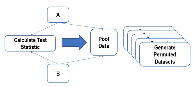
- Determinte the test statistics
- Observation is pooled, and new dataset is generated for every possible permutation of labels from groups
- Calculate the difference in means for each of these datasets
- Check where our test statistics falls in this distribution
- Advantage
- Very flexible
- No strict assumptions
- Widely applicable
- Drawbacks
- Computationally Expensive
- Custom coding required
Generating a single permutation
In the next few exercises, we will run a significance test using permutation testing. As discussed in the video, we want to see if there's any difference in the donations generated by the two designs - A and B. Suppose that you have been running both the versions for a few days and have generated 500 donations on A and 700 donations on B, stored in the variables donations_A and donations_B.
We first need to generate a null distribution for the difference in means. We will achieve this by generating multiple permutations of the dataset and calculating the difference in means for each case.
donations_A = np.array([7.15363286e+00, 2.02240490e+00, 1.54370448e+00, 4.80860209e+00,
       7.62642561e+00, 3.30058521e+00, 2.37058924e+01, 6.92785364e+00,
       3.93432116e+00, 2.98664221e+00, 2.52205350e+00, 7.83491938e+00,
       3.46363306e+00, 3.69196795e-01, 3.04542810e+00, 8.03635944e+00,
       1.20896556e+00, 1.15751776e+00, 4.54997304e+00, 4.55351188e+00,
       6.03730837e+00, 1.13600346e+01, 7.73403302e+00, 5.66541826e+00,
       7.69038204e+00, 2.34013992e+00, 2.69451474e+00, 1.55467056e+00,
       2.08641054e+00, 5.98136359e+00, 5.79758878e-01, 3.41180026e+00,
       3.38180211e+00, 4.08357880e+00, 3.32898159e+00, 2.24607719e+00,
       3.33442862e+00, 1.34314207e+01, 1.73115909e+01, 4.18096377e+00,
       5.86824609e+00, 7.37199778e-01, 2.29007093e+00, 3.21507841e+00,
       1.20733518e+01, 1.72973646e+00, 3.95867209e+00, 2.54264298e+01,
       4.39738249e+00, 5.69434848e+00, 7.71288120e-01, 1.05039631e+01,
       5.54382280e+00, 4.72564402e+00, 2.51827118e+00, 2.17547509e+00,
       3.23763715e+00, 6.86104476e+00, 1.24986178e+01, 4.28527304e+00,
       6.63951203e+00, 5.29041637e+00, 5.88343175e+00, 6.73784273e+00,
       1.10839795e+01, 5.21162799e-01, 8.65548290e+00, 1.67563618e+00,
       1.29568920e+00, 5.09820187e+00, 6.03647739e-01, 1.29940150e+01,
       5.92106741e+00, 7.71145201e+00, 9.75641890e-02, 5.41479857e+00,
       4.88220440e+00, 1.03869381e+00, 9.96827044e-01, 7.13508703e+00,
       2.30310027e+00, 7.06535435e+00, 4.84977600e+00, 2.95546458e+00,
       1.55522115e+01, 1.10584428e+01, 2.65337427e+00, 2.67420709e-01,
       2.18105869e+00, 3.04683794e+00, 7.32384225e+00, 3.22362829e+01,
       2.63954619e+00, 8.62673398e+00, 5.39626123e+00, 7.06012667e+00,
       9.83077347e-01, 3.05372718e+00, 1.65338197e+00, 2.52459352e+00,
       4.31852605e+00, 6.59091568e+00, 6.71682860e-01, 8.41747654e-01,
       2.33147632e+00, 6.50052761e+00, 1.12445716e+01, 4.83463539e+00,
       1.15635162e+01, 2.91521595e+00, 2.28569953e+00, 2.62419344e+00,
       1.12580302e+00, 1.06005037e+01, 2.48102160e+00, 4.82273069e+00,
       5.18434570e+00, 4.42300896e+00, 1.61501034e-02, 2.67123359e+01,
       1.41448824e+01, 1.39640533e+00, 2.07601611e+00, 4.40394197e+00,
       1.39313031e+01, 2.46741537e+01, 1.78673437e+00, 4.98562121e+00,
       9.86941707e+00, 3.00891678e+00, 7.87989267e+00, 1.05376100e+00,
       5.50823207e+00, 1.20534269e+01, 2.46342324e+01, 4.96154929e-01,
       3.35534157e+00, 1.37302986e+00, 3.59396956e+00, 4.76130100e+00,
       5.87838622e-01, 2.11320218e+00, 1.57519880e+01, 5.04993508e+00,
       3.66842994e+00, 8.40299238e+00, 8.12556925e+00, 2.98791942e-01,
       7.40035604e+00, 1.09671812e+01, 1.08868440e+00, 9.11204480e+00,
       2.02574498e+00, 2.19576255e+00, 6.56643327e+00, 7.08595672e-01,
       6.55946442e+00, 1.31278715e+01, 7.15051206e+00, 3.48242496e+00,
       3.45980981e+00, 8.69147259e+00, 5.00331722e+00, 5.32358877e-01,
       5.24328366e+00, 1.01193298e+01, 2.46648252e+00, 1.57513533e+01,
       8.33499890e+00, 5.12079461e+00, 8.35735220e+00, 4.94741963e-01,
       1.17705516e+01, 1.03391383e+01, 1.44391237e+01, 8.26139805e-01,
       5.11910163e-01, 8.93893365e-01, 3.05874406e+00, 3.31308303e+00,
       4.95621045e+00, 7.82316691e-01, 1.34936676e+00, 1.00165400e+01,
       3.78653060e+00, 9.89962880e+00, 4.47245483e-02, 4.81232019e+00,
       1.61235015e+01, 5.23616216e+00, 1.38475433e+00, 7.58993321e+00,
       2.85840847e+00, 6.62266468e+00, 1.78548820e-01, 6.06196626e+00,
       1.96366145e-01, 8.19379157e+00, 3.84233798e+00, 7.78973683e-01,
       4.69365326e+00, 4.14650118e-01, 6.35689533e+00, 3.32596743e+01,
       8.80235474e+00, 5.11671494e+00, 6.49757260e-01, 7.22051924e+00,
       6.49350287e+00, 3.02060141e-01, 9.42994312e+00, 4.38779385e+00,
       3.32937247e+00, 9.31231373e+00, 3.18177591e+00, 3.93541215e+00,
       1.20263585e+00, 2.32562353e+00, 1.12066487e+01, 1.24143472e+00,
       3.24040478e+00, 2.70780118e+01, 1.61983735e+00, 1.49213797e+01,
       1.50353699e+01, 5.74417482e-01, 3.73784056e+00, 4.18553823e+00,
       2.25837113e+00, 2.90980328e-01, 1.65994352e+00, 6.02434475e-01,
       1.63282042e+00, 9.89503444e+00, 1.35215290e+01, 2.65108930e-01,
       2.15676008e+00, 2.36493902e+01, 4.65271737e+00, 5.90596197e+00,
       3.33650476e-02, 3.98047533e+00, 2.67036496e+01, 2.82180310e+00,
       6.12449905e-01, 3.71836287e+00, 1.97817485e+01, 2.50975773e+00,
       9.62439620e+00, 9.62211685e+00, 1.40104465e+00, 3.51510242e+00,
       7.54426839e+00, 3.17108474e+00, 1.27178976e+00, 2.05580402e+01,
       6.31180998e+00, 1.20353557e+01, 1.53398466e-01, 1.86288656e+00,
       4.18378790e+00, 4.18986276e-01, 2.97996482e+01, 1.61875742e+00,
       2.81323057e+00, 1.44488187e+00, 6.68579156e-01, 1.58754277e+00,
       2.14528168e+00, 6.03798635e+00, 1.98132308e+00, 2.69910531e+00,
       3.57634362e-02, 2.73158042e+00, 4.57995000e+00, 1.06053646e+00,
       5.45936403e+00, 2.08164175e+00, 5.99885739e+00, 1.59275095e-01,
       1.31137990e+01, 9.74996914e-02, 8.14629899e-01, 9.00787380e+00,
       2.81890764e-01, 7.44794442e+00, 2.12523106e+01, 1.23195060e+01,
       7.43059158e+00, 1.90937799e+01, 3.37074897e+00, 1.23756913e+01,
       2.63994493e+00, 1.59353360e+01, 9.66491466e-01, 1.68833665e+01,
       1.07283809e+01, 1.12269530e+01, 7.93807822e-01, 5.44527793e+00,
       9.91699451e-02, 7.66322715e+00, 4.66056240e-02, 5.31822002e-01,
       1.53321340e+00, 1.24826299e+01, 2.71134462e+00, 4.65865018e+00,
       5.03741184e+00, 1.53294188e+00, 5.09385035e+00, 6.48967790e+00,
       2.12502900e+00, 3.25417493e+00, 3.62081435e+00, 1.61605062e+01,
       5.31302349e+00, 1.77682601e+01, 4.87205396e+00, 4.16562392e+00,
       2.12307837e-02, 3.93382578e+00, 1.57412892e+01, 1.32661648e+00,
       3.20981488e-01, 3.13312853e+00, 2.79507990e+00, 1.16758893e+01,
       1.61829606e-01, 1.51655745e+01, 6.85356086e+00, 1.40745838e+01,
       5.61175686e+00, 1.00263901e+01, 2.45271857e+00, 2.58069478e+00,
       2.96454098e+00, 8.43401504e+00, 2.76546583e+00, 1.66417151e+00,
       1.66517164e+01, 1.43165231e+01, 2.57360606e+00, 6.04120097e+00,
       1.91992769e+00, 1.38490096e+00, 2.45990759e+00, 2.37695034e+00,
       1.28364794e+01, 1.03660801e+01, 7.41945592e+00, 1.92158339e+01,
       3.29473146e+00, 1.68648774e+00, 7.49288469e-01, 2.14908525e+00,
       9.41773910e-01, 5.80295247e-01, 5.54188934e+00, 2.71710895e+00,
       4.98853210e+00, 1.27422858e+00, 6.77886925e+00, 1.45629390e+00,
       1.95457691e+00, 8.12320517e+00, 4.92231023e+00, 2.44633364e+00,
       4.69828406e+00, 7.10472113e+00, 1.45915258e+01, 5.21520083e+00,
       1.58915801e+00, 8.23902821e+00, 9.02422786e+00, 1.34187193e+00,
       1.03079618e+01, 3.75220064e+00, 9.07840601e+00, 1.62674524e+00,
       2.42601690e+00, 1.84353066e+01, 6.43442380e+00, 8.89360329e+00,
       6.99571578e+00, 1.37122934e+00, 3.81707186e+00, 9.93175632e+00,
       6.74422911e+00, 3.62767602e-02, 5.48796568e-01, 2.55518301e+00,
       1.73337149e+01, 4.05408935e+00, 1.88971342e+00, 2.68169630e+00,
       1.41929271e+00, 3.28079030e+00, 1.47567515e+00, 1.12151812e+01,
       3.65582148e+00, 1.96937478e+00, 1.62086806e+01, 2.26433976e+00,
       1.44286812e+01, 2.66333158e-01, 7.36785267e+00, 3.96860098e+00,
       3.52430794e+00, 2.21996761e-01, 2.49203428e-01, 2.42757547e+00,
       1.76383283e+01, 5.76866972e+00, 2.76150652e+00, 5.68014458e+00,
       1.38502497e+00, 1.08241878e+00, 2.69478371e+00, 1.19421414e+01,
       4.27277801e+00, 2.11354984e+00, 1.80046649e+01, 1.01558115e+01,
       2.34027311e+00, 2.14743942e+01, 2.62211091e+01, 3.15218614e+00,
       6.40134065e+00, 3.12175373e+00, 1.78516715e+00, 5.17614704e-01,
       1.83597528e+00, 1.90043999e+00, 3.05135995e+00, 1.22656402e+00,
       1.84510434e+01, 6.51393113e-01, 5.88831298e+00, 3.49712489e+00,
       3.30486749e+00, 2.79121217e+00, 1.21640422e+01, 1.97500056e+00,
       1.24744775e-01, 1.50133191e+01, 1.19918286e+01, 1.94526138e+00,
       4.44756855e+00, 6.93059059e-01, 5.88502790e-01, 1.09012124e+01,
       3.16849927e+00, 6.50322658e+00, 1.72093727e+01, 1.68726308e+00,
       7.94831348e-02, 1.46668555e-01, 7.41454977e+00, 1.55058604e+01,
       3.77912218e+00, 2.82106969e+00, 4.69659911e+00, 1.17504345e+01,
       6.33597038e+00, 1.59145361e+00, 8.93874514e+00, 8.67474288e-01,
       1.08596642e+00, 5.69105969e+00, 1.63702407e+00, 7.32017711e+00,
       2.58025478e+00, 1.94959571e+00, 4.09759162e+01, 2.48783982e-01,
       6.22774284e+00, 2.36809873e-01, 8.56795689e+00, 1.56888959e+00,
       5.64755610e-01, 6.27241507e+00, 7.91408500e+00, 6.80099872e+00,
       3.19777776e-01, 2.09144942e+00, 3.59890663e+00, 2.03051241e+00,
       9.98062360e+00, 8.43267717e-01, 5.68327391e+00, 2.66455378e+01,
       1.39708977e+01, 1.50738393e+00, 4.91345800e-04, 2.36540713e+01,
       1.28587874e+01, 1.51149367e+01, 3.22202744e+00, 8.18990927e+00])

donations_B = np.array([1.19656474e+00, 2.49040320e+00, 9.53746976e+00, 6.82606285e-01,
       1.12152344e+01, 3.43093700e+00, 2.77646272e+00, 1.82386960e+00,
       1.24354723e+01, 3.64515134e+00, 8.14887581e+00, 9.74739510e+00,
       1.27798024e+01, 1.80758132e+00, 2.07614450e+00, 4.52025320e+00,
       2.91092911e+00, 1.35035758e+01, 2.53386965e+00, 3.24831293e+00,
       4.80103139e+00, 2.59378065e+00, 2.44499059e+01, 5.20424895e-01,
       1.24617571e+00, 1.94787364e+00, 7.99217521e-01, 1.67190676e+00,
       7.55351558e+00, 3.70006200e+00, 1.72717251e-01, 2.02629196e+01,
       4.78564798e+00, 3.03739127e-01, 5.41126574e+00, 2.37704603e+00,
       7.29022267e-01, 4.14672025e+00, 6.49288193e+00, 5.56041209e+00,
       1.42185881e+00, 3.72079438e+00, 3.85731089e+00, 6.30806898e+00,
       2.23039928e+00, 7.99082335e+00, 4.94325682e+00, 1.95427968e-01,
       3.95356876e+00, 9.89932403e+00, 4.19172221e+00, 9.66881775e-01,
       3.57059143e+00, 7.07235483e+00, 5.83260107e-01, 8.49405343e+00,
       9.16500024e-01, 3.81866902e+00, 2.43671329e+00, 1.42924389e+00,
       5.21256611e+00, 1.90545622e-01, 7.13653618e+00, 3.74267199e+00,
       1.04281517e+01, 3.67733398e+00, 1.78307749e-01, 7.75094268e-01,
       7.93849435e+00, 3.38613342e+00, 2.91589990e+00, 1.91681667e+00,
       1.67421222e+00, 1.68902829e+01, 2.83670943e+00, 1.07709562e+01,
       5.22293814e+00, 9.77472179e+00, 9.56792546e+00, 1.56534123e+01,
       5.98568505e+00, 8.18396681e+00, 6.60492872e+00, 4.64721974e+00,
       6.31780261e+00, 6.28951297e+00, 2.08840298e-01, 3.62949699e+00,
       7.86676827e+00, 1.39171038e+00, 3.12882590e+00, 2.85452129e+00,
       2.57740864e+00, 6.49629659e-01, 3.72969790e+00, 2.95519503e+00,
       5.44419240e+00, 3.98602116e+00, 1.39646740e-01, 1.62192359e-01,
       6.04257889e+00, 6.14783990e+00, 1.60867766e+01, 1.04658642e+01,
       3.15611976e+00, 4.91624772e+00, 3.05490344e+00, 1.26122869e+00,
       2.36345216e+00, 5.48428348e-01, 5.49096867e+00, 1.06615264e+00,
       3.22624219e+00, 1.71228321e+01, 1.60906182e-01, 8.22781194e-01,
       1.77323632e+00, 1.42199480e+01, 1.19757939e+01, 8.83690909e-01,
       1.98476709e+01, 6.94644470e+00, 3.88239486e+00, 1.34194386e+01,
       1.06266795e+01, 2.48228419e+00, 5.34055891e+00, 5.21189441e+00,
       1.97981339e+00, 9.88537628e-01, 3.14438608e+00, 1.52774392e+00,
       2.19302969e+00, 1.54112427e+01, 3.09147765e+00, 5.77419073e+00,
       2.04909708e+00, 2.74366001e+01, 5.37595763e+00, 1.09083892e+00,
       5.16723847e-01, 1.43393848e+01, 1.44819541e+01, 4.85542938e+00,
       8.56875560e-02, 1.27791331e+00, 8.07921149e+00, 1.04156348e+01,
       3.02558824e+00, 2.27475244e+00, 1.60257623e+00, 6.21983428e-01,
       6.15046358e-01, 1.52459499e+01, 8.26763125e+00, 9.00296751e-01,
       1.15997587e+00, 5.32905419e+00, 7.23370957e+00, 8.31194831e+00,
       8.91673722e-01, 2.07160844e+01, 1.29257185e+00, 4.45086681e+00,
       4.42899866e+00, 1.71113726e+01, 5.35986313e+00, 4.39623051e+00,
       3.65707656e+00, 7.23356770e+00, 5.60556592e-01, 1.04704613e-02,
       1.52339562e+01, 3.45233068e+00, 1.98998069e+00, 2.29475080e+00,
       8.14420766e+00, 2.40933025e+00, 7.35205890e+00, 2.90321920e+00,
       9.29197976e+00, 3.96320401e-01, 3.28049343e+00, 3.14475962e+00,
       1.53485442e+00, 1.43777379e+01, 1.17708899e+01, 2.93130586e+00,
       5.11047459e-01, 1.15829319e+00, 1.58378224e+00, 3.31037261e+00,
       2.06529770e+00, 7.43911270e+00, 3.23157187e+00, 1.02153747e+01,
       2.73416748e+01, 1.24125530e+00, 4.72951666e+00, 9.40302917e+00,
       1.45236691e+01, 1.71306021e+00, 6.49220034e+00, 7.56501614e-02,
       1.05657130e+01, 3.30370760e-01, 6.60994306e+00, 2.61164084e+01,
       3.47764789e+00, 1.17439819e+00, 4.51494278e+00, 4.89282549e+00,
       5.51419711e+00, 9.47406084e-01, 1.14489709e+01, 4.85098149e+00,
       2.22731609e-01, 5.76071513e+00, 1.09130275e+00, 1.38607479e-01,
       4.00314166e+00, 8.39162641e+00, 9.82846288e+00, 5.46401636e-01,
       5.43899659e+00, 6.19066892e+00, 1.74436298e+00, 1.77654528e+01,
       1.63341384e+00, 3.62757709e-01, 3.66235525e+00, 5.92599873e+00,
       1.40293509e+00, 2.06684785e+00, 4.14630075e+00, 1.08876171e+01,
       6.87827393e+00, 1.17602980e+00, 1.45027156e+00, 3.71043402e+00,
       7.32579387e+00, 4.82165423e+00, 3.47899613e+00, 4.54564891e+00,
       7.05416552e+00, 3.85100290e+00, 1.14018066e+01, 1.46936879e+01,
       1.23464171e+01, 7.02266520e+00, 1.41394368e+00, 2.43287242e+00,
       1.64252000e+00, 5.35975794e+00, 1.95945052e+00, 7.02008451e+00,
       6.02421971e-01, 7.46638680e+00, 4.40826278e+00, 9.02084132e+00,
       2.81828166e+00, 4.90367233e+00, 4.04180408e+00, 1.85804859e+01,
       7.04217618e+00, 3.93523752e+00, 9.55996784e-01, 1.17229878e+01,
       1.15233767e+00, 5.24972861e+00, 1.37813611e+01, 1.26530596e+00,
       1.28042313e+00, 9.54660087e+00, 8.79128574e+00, 2.16703449e+00,
       1.54007897e+00, 6.81324038e-01, 2.20876901e+01, 9.01945685e+00,
       1.14825979e+01, 3.60443525e+00, 6.07363853e-01, 2.70065678e-01,
       2.00673377e+00, 1.26493381e+01, 1.47425105e+01, 9.19941105e+00,
       8.63910869e-01, 2.72297360e+00, 1.41342568e+00, 1.14926615e+00,
       5.77314968e+00, 3.32874645e+00, 1.96454369e+00, 5.27994178e-01,
       3.93468966e+00, 2.13108335e+00, 2.48047170e+00, 1.85900630e+00,
       2.44854418e+00, 4.05807258e+00, 7.12239124e-02, 9.40777525e+00,
       1.27500978e+01, 3.99842740e+00, 1.56001807e+00, 2.31468022e+01,
       2.41600389e+00, 5.91522324e+00, 5.85514960e+00, 2.84853700e+00,
       1.11045901e+00, 1.69929104e+01, 3.29047893e-01, 3.31939247e+00,
       1.24699303e+00, 1.74051701e+00, 8.81665669e+00, 2.28852238e+00,
       4.35138357e-01, 1.09270209e+00, 9.84391818e+00, 1.88675810e+01,
       1.55975197e+00, 5.62594656e+00, 4.23428585e-01, 6.42710012e+00,
       2.69301100e+00, 1.25149408e+01, 1.86646248e+00, 1.41908227e+01,
       3.49831609e+00, 2.14540586e+00, 5.20671367e+00, 1.43671867e+00,
       1.30528897e+00, 1.09293502e+00, 1.60818403e+01, 3.39537064e+00,
       6.96387584e+00, 3.21219316e+00, 4.42808218e+00, 4.38702082e+00,
       1.95317725e+01, 5.51962876e+00, 1.37066782e+00, 7.65716357e-02,
       1.23386610e+00, 3.03961706e+00, 2.49959605e+00, 8.36525070e+00,
       7.69855084e+00, 4.66588654e-01, 1.51838886e+01, 3.74812924e+00,
       4.53670405e+00, 2.59644646e+00, 5.24198650e+00, 1.02523778e+01,
       5.60330748e+00, 1.75492405e+01, 6.03860325e+00, 8.62202031e+00,
       2.30426942e-01, 5.58436779e+00, 5.31747073e+00, 5.36512283e-01,
       9.23807883e+00, 4.76182326e+00, 5.17522808e-01, 4.51276660e+00,
       3.25442326e+00, 1.32825651e+00, 9.97692556e-02, 2.27512018e+00,
       4.83596101e+00, 1.99701112e+00, 1.83546406e+00, 6.95394709e+00,
       7.10701039e+00, 6.34283815e+00, 5.33373306e-01, 3.63006659e+00,
       4.07994991e+00, 6.82862733e+00, 1.16743908e+01, 2.30255506e+00,
       2.79888439e+00, 6.59818092e+00, 5.43297027e+00, 4.08075549e+00,
       2.15498879e+00, 1.08675397e+00, 1.01552444e+00, 4.25520297e-01,
       4.23438666e-01, 9.34746649e+00, 2.41988603e+00, 3.13312732e-01,
       1.13373289e+01, 1.26331545e+00, 1.56072383e+00, 1.08144697e+00,
       1.71327390e+01, 5.96959631e-01, 6.40360770e+00, 1.34477674e+01,
       5.51312106e+00, 9.78529163e+00, 1.38830956e+00, 5.60318499e+00,
       6.03440749e+00, 3.06551479e+00, 1.02221337e+01, 5.92716369e+00,
       1.12631586e+01, 6.99597313e+00, 3.67287201e+00, 3.45263524e+00,
       3.02318788e+00, 1.09422966e-01, 3.83011003e+00, 2.74933312e+00,
       8.57107471e-01, 6.33883845e-01, 2.98329646e+00, 2.03657147e-01,
       2.15550044e+01, 2.37504814e+00, 2.40721762e+00, 2.62397886e-01,
       2.78148941e+00, 7.93535674e-02, 1.52778707e-01, 2.07075788e+00,
       8.60098006e+00, 3.07002667e+00, 7.47590119e-02, 8.90970622e-01,
       6.73388234e+00, 6.70266269e+00, 7.02275821e+00, 2.16677245e+00,
       2.17146031e+00, 8.09935239e+00, 2.53863453e+00, 6.49491690e+00,
       4.35088990e+00, 2.26547046e+00, 4.16943480e-01, 6.17200275e-01,
       1.10163567e+01, 3.01050777e+00, 2.55837629e+01, 2.26197349e+00,
       1.43810574e+00, 2.15806492e+00, 2.10101157e+00, 5.07167830e+00,
       6.40969098e-02, 7.20414636e+00, 2.69282261e+00, 2.83027532e+00,
       3.28036515e+00, 2.98203057e+00, 3.44050864e+00, 2.12250812e+00,
       3.01969734e+00, 2.59304027e+00, 3.65157428e+00, 4.88112050e+00,
       1.37903502e+00, 3.55082736e+00, 4.51467557e+00, 8.54679048e-02,
       3.67499163e+00, 1.36753669e+00, 2.59209312e+00, 8.75875771e+00,
       1.97437390e+00, 3.30066037e+00, 1.25261799e-01, 1.84627498e+00,
       5.10438403e+00, 1.89286318e+00, 1.15208410e+00, 1.71707114e+00,
       1.54368597e+01, 4.54011799e-01, 3.11211816e+00, 3.00804073e-01,
       3.86808084e+00, 7.89329663e-01, 5.02676840e+00, 1.53532668e+00,
       5.87070109e+00, 2.13200925e+00, 2.08860049e-02, 1.74704069e+00,
       4.27214524e-01, 3.41637666e+00, 1.70464123e+00, 5.10814331e+00,
       3.46509542e+00, 1.83552565e-01, 1.91827763e+00, 3.35750764e+00,
       4.24554232e+00, 5.53938827e-01, 5.24870050e+00, 2.10566870e+00,
       1.01009927e+00, 8.18216225e+00, 3.55457791e-01, 1.32798881e+01,
       6.12540614e+00, 3.22741702e+00, 5.61181745e-02, 2.47250885e+00,
       5.18944537e+00, 9.79189626e+00, 4.80858522e+00, 2.53505970e+00,
       2.96523687e+00, 1.03294815e+01, 2.16436634e+00, 3.36886593e-01,
       2.92301171e+00, 3.23770275e+01, 2.38834759e+00, 1.07249708e+00,
       2.30901082e-01, 9.37487942e-01, 1.95828740e+00, 4.26984758e+00,
       5.47691378e+00, 2.18813468e-01, 1.37584514e+01, 1.34357116e+00,
       8.07080088e-01, 3.78394448e+00, 5.65959142e+00, 1.83545061e+00,
       5.53485390e+00, 1.74278175e+00, 1.16226977e+01, 1.06303492e+01,
       3.69278971e-01, 8.14962974e-01, 5.98761303e+00, 6.00543509e-04,
       8.62462585e+00, 2.20214501e+00, 6.82501117e+00, 2.26227605e-01,
       1.17395832e+00, 3.67184262e-01, 9.91180389e-01, 2.42596184e+00,
       3.38195979e+00, 1.23901335e+01, 4.93321755e+00, 6.12904433e+00,
       4.28392292e-01, 1.68987645e+00, 2.39767605e+01, 4.10970395e+00,
       7.75154106e+00, 1.65108656e-01, 4.39110605e-01, 5.78363060e-01,
       7.70193861e-02, 1.27538843e+01, 1.46270453e+00, 2.83747087e+01,
       6.69953255e+00, 1.44248396e+00, 2.40209331e+01, 1.01450297e+01,
       9.01605827e-01, 1.02481113e+00, 5.70008072e+00, 4.07570278e-01,
       4.39166252e+00, 3.44622894e-01, 1.25063171e+00, 1.48250410e+01,
       3.45147264e+00, 4.26321190e+00, 1.57138486e+00, 2.89964291e+00,
       7.13595387e-01, 3.63472276e+00, 2.77329902e-01, 2.47261101e-01,
       5.69167037e+00, 2.82754459e-01, 3.68323718e+00, 1.54641173e+00,
       1.03939046e+00, 4.25859180e+00, 1.75817616e+00, 3.04754587e+00,
       7.48151951e-01, 6.76153827e-01, 5.63206643e-01, 3.71248209e-01,
       4.03397323e+00, 7.05304780e+00, 7.85991283e+00, 1.58319871e+01,
       9.21972681e-01, 7.28707909e-01, 3.17396477e+00, 9.86667744e+00,
       7.28507091e+00, 4.08424219e+00, 8.52656276e-01, 2.48184126e+00,
       6.35315945e+00, 2.33733572e+00, 1.99525358e-01, 4.38395559e+00,
       6.36723217e+00, 6.27232318e+00, 9.00814473e-01, 2.04730232e+00,
       2.63115415e+00, 2.72778771e+00, 6.06086132e-01, 2.43498831e+00,
       3.53250156e+00, 6.19904790e+00, 4.21343225e+00, 2.59538588e+00,
       1.31275628e+01, 4.55755545e+00, 1.84027480e+01, 1.01011995e+01,
       5.59855814e+00, 1.14787175e+01, 2.36876132e+01, 1.24793347e+00,
       5.87298466e+00, 1.25529243e+01, 8.77666105e-02, 8.03443077e+00,
       4.68273978e-01, 1.24177956e+01, 4.73392204e+00, 8.84100221e-01,
       2.01038872e-01, 8.79611728e+00, 7.51161489e-01, 1.40289801e+01,
       4.76309817e-01, 9.10013068e+00, 2.75418195e+00, 1.03074324e+01,
       7.31748078e+00, 9.58261106e+00, 3.17667577e+00, 6.25476857e+00,
       1.91852488e+00, 2.41611024e-01, 1.32243330e+00, 6.81283489e-03,
       2.25514913e+00, 3.40440200e+00, 9.79893882e-02, 3.87992255e-02,
       5.79919858e+00, 5.29224509e-01, 3.83571092e-01, 3.42191029e+00,
       6.33206648e+00, 1.88973564e+01, 1.75060591e+00, 6.25084288e-01,
       3.54991820e-01, 1.16288135e+00, 5.27106238e-01, 1.69505065e-02,
       1.67787904e+00, 8.96870825e-01, 9.20924290e-02, 2.18967278e+00,
       8.74108057e+00, 1.80959704e+00, 6.19109167e+00, 6.52329442e+00,
       1.29443515e-01, 1.63226493e+01, 7.48358420e-01, 6.31976402e+00,
       2.38569017e+00, 1.01332035e+01, 2.64527664e+01, 1.07415949e+00])
np.random.seed(123)

# Concatenate the two arrays donations_A and donations_B into data
len_A, len_B = len(donations_A), len(donations_B)
data = np.concatenate([donations_A, donations_B])

# Get a single permutation of the concatenated length
perm = np.random.permutation(len(donations_A) + len(donations_B))

# Calculate the permutated datasets and difference in means
permuted_A = data[perm[:len(donations_A)]]
permuted_B = data[perm[len(donations_A):]]
diff_in_means = np.mean(permuted_A) - np.mean(permuted_B)
print("Difference in the permuted mean values = {}.".format(diff_in_means))
Hypothesis testing - Difference of means
We want to test the hypothesis that there is a difference in the average donations received from A and B. Previously, you learned how to generate one permutation of the data. Now, we will generate a null distribution of the difference in means and then calculate the p-value.
For the null distribution, we first generate multiple permuted datasets and store the difference in means for each case. We then calculate the test statistic as the difference in means with the original dataset. Finally, we calculate the p-value as twice the fraction of cases where the difference is greater than or equal to the absolute value of the test statistic (2-sided hypothesis). A p-value of less than say 0.05 could then determine statistical significance.
reps = 1000
np.random.seed(123)

# Generate permutations equal to the number of repetitions
perm = np.array([np.random.permutation(len(donations_A) + len(donations_B)) for i in range(reps)])
permuted_A_datasets = data[perm[:, :len(donations_A)]]
permuted_B_datasets = data[perm[:, len(donations_A):]]

# Calculate the difference in means for each of the datasets
samples = np.mean(permuted_A_datasets, axis=1) - np.mean(permuted_B_datasets, axis=1)

# Calculate the test statistic and p-value
test_stat = np.mean(donations_A) - np.mean(donations_B)
p_val = 2*np.sum(samples >= np.abs(test_stat))/reps
print("p-value = {}".format(p_val))
Hypothesis testing - Non-standard statistics
In the previous two exercises, we ran a permutation test for the difference in mean values. Now let's look at non-standard statistics.
Suppose that you're interested in understanding the distribution of the donations received from websites A and B. For this, you want to see if there's a statistically significant difference in the median and the 80th percentile of the donations. Permutation testing gives you a wonderfully flexible framework for attacking such problems.
Let's go through running a test to see if there's a difference in the median and the 80th percentile of the distribution of donations. As before, you're given the donations from the websites A and B in the variables donations_A and donations_B respectively.
np.random.seed(123)

# Calculate the difference in 80th percentile and median for each of the permuted datasets (A and B)
samples_percentile = np.percentile(permuted_A_datasets, 80, axis=1) \
                        - np.percentile(permuted_B_datasets, 80, axis=1)
samples_median = np.median(permuted_A_datasets, axis=1) - np.median(permuted_B_datasets, axis=1)
test_stat_percentile = np.percentile(donations_A, 80) \
                        - np.percentile(donations_B, 80)
test_stat_median = np.median(donations_A) - np.median(donations_B)
p_val_percentile = 2 * np.sum(samples_percentile >= np.abs(test_stat_percentile)) / reps
p_val_median = 2 * np.sum(samples_median >= np.abs(test_stat_median)) / reps

print("80th Percentile: test statistic = {}, p-value = {}".format(test_stat_percentile, p_val_percentile))
print("Median: test statistic = {}, p-value = {}".format(test_stat_median, p_val_median))