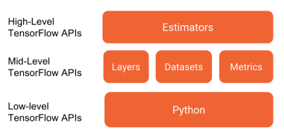
import tensorflow as tf
import pandas as pd
import numpy as np
import matplotlib.pyplot as plt

plt.rcParams['figure.figsize'] = (8, 8)
tf.__version__
'2.2.0'

Defining neural networks with Keras

The sequential model in Keras

n chapter 3, we used components of the keras API in tensorflow to define a neural network, but we stopped short of using its full capabilities to streamline model definition and training. In this exercise, you will use the keras sequential model API to define a neural network that can be used to classify images of sign language letters. You will also use the .summary() method to print the model's architecture, including the shape and number of parameters associated with each layer.

Note that the images were reshaped from (28, 28) to (784,), so that they could be used as inputs to a dense layer.

model = tf.keras.Sequential()

# Define the first dense layer
model.add(tf.keras.layers.Dense(16, activation='relu', input_shape=(784,)))

# Define the second dense layer
model.add(tf.keras.layers.Dense(8, activation='relu', ))

# Define the output layer
model.add(tf.keras.layers.Dense(4, activation='softmax'))

# Print the model architecture
print(model.summary())
Model: "sequential"
_________________________________________________________________
Layer (type)                 Output Shape              Param #   
=================================================================
dense (Dense)                (None, 16)                12560     
_________________________________________________________________
dense_1 (Dense)              (None, 8)                 136       
_________________________________________________________________
dense_2 (Dense)              (None, 4)                 36        
=================================================================
Total params: 12,732
Trainable params: 12,732
Non-trainable params: 0
_________________________________________________________________
None

Notice that we've defined a model, but we haven't compiled it. The compilation step in keras allows us to set the optimizer, loss function, and other useful training parameters in a single line of code. Furthermore, the .summary() method allows us to view the model's architecture.

Compiling a sequential model

In this exercise, you will work towards classifying letters from the Sign Language MNIST dataset; however, you will adopt a different network architecture than what you used in the previous exercise. There will be fewer layers, but more nodes. You will also apply dropout to prevent overfitting. Finally, you will compile the model to use the adam optimizer and the categorical_crossentropy loss. You will also use a method in keras to summarize your model's architecture.

model = tf.keras.Sequential()

# Define the first dense layer
model.add(tf.keras.layers.Dense(16, activation='sigmoid', input_shape=(784,)))

# Apply dropout to the first layer's output
model.add(tf.keras.layers.Dropout(0.25))

# Define the output layer
model.add(tf.keras.layers.Dense(4, activation='softmax'))

# Compile the model
model.compile(optimizer='adam', loss='categorical_crossentropy')

# Print a model summary
print(model.summary())
Model: "sequential_1"
_________________________________________________________________
Layer (type)                 Output Shape              Param #   
=================================================================
dense_3 (Dense)              (None, 16)                12560     
_________________________________________________________________
dropout (Dropout)            (None, 16)                0         
_________________________________________________________________
dense_4 (Dense)              (None, 4)                 68        
=================================================================
Total params: 12,628
Trainable params: 12,628
Non-trainable params: 0
_________________________________________________________________
None

Defining a multiple input model

In some cases, the sequential API will not be sufficiently flexible to accommodate your desired model architecture and you will need to use the functional API instead. If, for instance, you want to train two models with different architectures jointly, you will need to use the functional API to do this. In this exercise, we will see how to do this. We will also use the .summary() method to examine the joint model's architecture.

m1_inputs = tf.keras.Input(shape=(784,))
m2_inputs = tf.keras.Input(shape=(784,))
m1_layer1 = tf.keras.layers.Dense(12, activation='sigmoid')(m1_inputs)
m1_layer2 = tf.keras.layers.Dense(4, activation='softmax')(m1_layer1)

# For model 2, pass the input layer to layer 1 and layer 1 to layer 2
m2_layer1 = tf.keras.layers.Dense(12, activation='relu')(m2_inputs)
m2_layer2 = tf.keras.layers.Dense(4, activation='softmax')(m2_layer1)

# Merge model outputs and define a functional model
merged = tf.keras.layers.add([m1_layer2, m2_layer2])
model = tf.keras.Model(inputs=[m1_inputs, m2_inputs], outputs=merged)

# Print a model summary
print(model.summary())
Model: "model"
__________________________________________________________________________________________________
Layer (type)                    Output Shape         Param #     Connected to                     
==================================================================================================
input_1 (InputLayer)            [(None, 784)]        0                                            
__________________________________________________________________________________________________
input_2 (InputLayer)            [(None, 784)]        0                                            
__________________________________________________________________________________________________
dense_5 (Dense)                 (None, 12)           9420        input_1[0][0]                    
__________________________________________________________________________________________________
dense_7 (Dense)                 (None, 12)           9420        input_2[0][0]                    
__________________________________________________________________________________________________
dense_6 (Dense)                 (None, 4)            52          dense_5[0][0]                    
__________________________________________________________________________________________________
dense_8 (Dense)                 (None, 4)            52          dense_7[0][0]                    
__________________________________________________________________________________________________
add (Add)                       (None, 4)            0           dense_6[0][0]                    
                                                                 dense_8[0][0]                    
==================================================================================================
Total params: 18,944
Trainable params: 18,944
Non-trainable params: 0
__________________________________________________________________________________________________
None

Notice that the .summary() method yields a new column: connected to. This column tells you how layers connect to each other within the network. We can see that dense_9, for instance, is connected to the input_2 layer. We can also see that the add layer, which merged the two models, connected to both dense_10 and dense_12.

Training and validation with Keras

Training with Keras

In this exercise, we return to our sign language letter classification problem. We have 2000 images of four letters--A, B, C, and D--and we want to classify them with a high level of accuracy. We will complete all parts of the problem, including the model definition, compilation, and training.

df = pd.read_csv('./dataset/slmnist.csv', header=None)
X = df.iloc[:, 1:]
y = df.iloc[:, 0]
sign_language_features = (X -  X.mean()) / (X.max() - X.min()).to_numpy()
sign_language_labels = pd.get_dummies(y).astype(np.float32).to_numpy()
model = tf.keras.Sequential()

# Define a hidden layer
model.add(tf.keras.layers.Dense(16, activation='relu', input_shape=(784, )))

# Define the output layer
model.add(tf.keras.layers.Dense(4, activation='softmax'))

# Compile the model
model.compile(optimizer='SGD', loss='categorical_crossentropy')

# Complete the fitting operation
model.fit(sign_language_features, sign_language_labels, epochs=5)
Epoch 1/5
63/63 [==============================] - 0s 1ms/step - loss: 1.2644
Epoch 2/5
63/63 [==============================] - 0s 1ms/step - loss: 1.0355
Epoch 3/5
63/63 [==============================] - 0s 988us/step - loss: 0.8604
Epoch 4/5
63/63 [==============================] - 0s 960us/step - loss: 0.7198
Epoch 5/5
63/63 [==============================] - 0s 911us/step - loss: 0.5997
<tensorflow.python.keras.callbacks.History at 0x7f76000c0c50>

You probably noticed that your only measure of performance improvement was the value of the loss function in the training sample, which is not particularly informative.

Metrics and validation with Keras

We trained a model to predict sign language letters in the previous exercise, but it is unclear how successful we were in doing so. In this exercise, we will try to improve upon the interpretability of our results. Since we did not use a validation split, we only observed performance improvements within the training set; however, it is unclear how much of that was due to overfitting. Furthermore, since we did not supply a metric, we only saw decreases in the loss function, which do not have any clear interpretation.

model = tf.keras.Sequential()

# Define the first layer
model.add(tf.keras.layers.Dense(32, activation='sigmoid', input_shape=(784,)))

# Add activation function to classifier
model.add(tf.keras.layers.Dense(4, activation='softmax'))

# Set the optimizer, loss function, and metrics
model.compile(optimizer='RMSprop', loss='categorical_crossentropy', metrics=['accuracy'])

# Add the number of epochs and the validation split
model.fit(sign_language_features, sign_language_labels, epochs=10, validation_split=0.1)
Epoch 1/10
57/57 [==============================] - 0s 3ms/step - loss: 0.9454 - accuracy: 0.7244 - val_loss: 0.5956 - val_accuracy: 0.8550
Epoch 2/10
57/57 [==============================] - 0s 2ms/step - loss: 0.4391 - accuracy: 0.9439 - val_loss: 0.3207 - val_accuracy: 0.9800
Epoch 3/10
57/57 [==============================] - 0s 2ms/step - loss: 0.2457 - accuracy: 0.9889 - val_loss: 0.1868 - val_accuracy: 0.9850
Epoch 4/10
57/57 [==============================] - 0s 2ms/step - loss: 0.1399 - accuracy: 0.9939 - val_loss: 0.1073 - val_accuracy: 0.9950
Epoch 5/10
57/57 [==============================] - 0s 2ms/step - loss: 0.0796 - accuracy: 0.9983 - val_loss: 0.0614 - val_accuracy: 1.0000
Epoch 6/10
57/57 [==============================] - 0s 2ms/step - loss: 0.0446 - accuracy: 0.9989 - val_loss: 0.0346 - val_accuracy: 1.0000
Epoch 7/10
57/57 [==============================] - 0s 2ms/step - loss: 0.0243 - accuracy: 1.0000 - val_loss: 0.0191 - val_accuracy: 1.0000
Epoch 8/10
57/57 [==============================] - 0s 2ms/step - loss: 0.0134 - accuracy: 1.0000 - val_loss: 0.0109 - val_accuracy: 1.0000
Epoch 9/10
57/57 [==============================] - 0s 2ms/step - loss: 0.0073 - accuracy: 1.0000 - val_loss: 0.0059 - val_accuracy: 1.0000
Epoch 10/10
57/57 [==============================] - 0s 2ms/step - loss: 0.0041 - accuracy: 1.0000 - val_loss: 0.0033 - val_accuracy: 1.0000
<tensorflow.python.keras.callbacks.History at 0x7f75a877b390>

With the keras API, you only needed 14 lines of code to define, compile, train, and validate a model. You may have noticed that your model performed quite well. In just 10 epochs, we achieved a classification accuracy of over 90% in the validation sample!

Overfitting detection

In this exercise, we'll work with a small subset of the examples from the original sign language letters dataset. A small sample, coupled with a heavily-parameterized model, will generally lead to overfitting. This means that your model will simply memorize the class of each example, rather than identifying features that generalize to many examples.

You will detect overfitting by checking whether the validation sample loss is substantially higher than the training sample loss and whether it increases with further training. With a small sample and a high learning rate, the model will struggle to converge on an optimum. You will set a low learning rate for the optimizer, which will make it easier to identify overfitting.

model = tf.keras.Sequential()

# Define the first layer
model.add(tf.keras.layers.Dense(1024, activation='relu', input_shape=(784, )))

# Add activation function to classifier
model.add(tf.keras.layers.Dense(4, activation='softmax'))

# Finish the model compilation
model.compile(optimizer=tf.keras.optimizers.Adam(lr=0.001),
              loss='categorical_crossentropy', metrics=['accuracy'])

# Complete the model fit operation
model.fit(sign_language_features, sign_language_labels, epochs=50, validation_split=0.5)
Epoch 1/50
32/32 [==============================] - 0s 5ms/step - loss: 0.3319 - accuracy: 0.8980 - val_loss: 0.0688 - val_accuracy: 0.9760
Epoch 2/50
32/32 [==============================] - 0s 3ms/step - loss: 0.0194 - accuracy: 0.9980 - val_loss: 0.0228 - val_accuracy: 0.9920
Epoch 3/50
32/32 [==============================] - 0s 3ms/step - loss: 0.0071 - accuracy: 0.9990 - val_loss: 0.0180 - val_accuracy: 0.9940
Epoch 4/50
32/32 [==============================] - 0s 3ms/step - loss: 0.0038 - accuracy: 1.0000 - val_loss: 0.0071 - val_accuracy: 1.0000
Epoch 5/50
32/32 [==============================] - 0s 3ms/step - loss: 0.0024 - accuracy: 1.0000 - val_loss: 0.0050 - val_accuracy: 1.0000
Epoch 6/50
32/32 [==============================] - 0s 3ms/step - loss: 0.0018 - accuracy: 1.0000 - val_loss: 0.0051 - val_accuracy: 1.0000
Epoch 7/50
32/32 [==============================] - 0s 3ms/step - loss: 0.0013 - accuracy: 1.0000 - val_loss: 0.0043 - val_accuracy: 1.0000
Epoch 8/50
32/32 [==============================] - 0s 3ms/step - loss: 0.0011 - accuracy: 1.0000 - val_loss: 0.0035 - val_accuracy: 1.0000
Epoch 9/50
32/32 [==============================] - 0s 3ms/step - loss: 8.9295e-04 - accuracy: 1.0000 - val_loss: 0.0035 - val_accuracy: 1.0000
Epoch 10/50
32/32 [==============================] - 0s 3ms/step - loss: 7.4761e-04 - accuracy: 1.0000 - val_loss: 0.0027 - val_accuracy: 1.0000
Epoch 11/50
32/32 [==============================] - 0s 3ms/step - loss: 6.3920e-04 - accuracy: 1.0000 - val_loss: 0.0027 - val_accuracy: 1.0000
Epoch 12/50
32/32 [==============================] - 0s 3ms/step - loss: 5.5781e-04 - accuracy: 1.0000 - val_loss: 0.0021 - val_accuracy: 1.0000
Epoch 13/50
32/32 [==============================] - 0s 3ms/step - loss: 4.8971e-04 - accuracy: 1.0000 - val_loss: 0.0023 - val_accuracy: 1.0000
Epoch 14/50
32/32 [==============================] - 0s 3ms/step - loss: 4.2039e-04 - accuracy: 1.0000 - val_loss: 0.0020 - val_accuracy: 1.0000
Epoch 15/50
32/32 [==============================] - 0s 3ms/step - loss: 3.7444e-04 - accuracy: 1.0000 - val_loss: 0.0019 - val_accuracy: 1.0000
Epoch 16/50
32/32 [==============================] - 0s 3ms/step - loss: 3.3658e-04 - accuracy: 1.0000 - val_loss: 0.0018 - val_accuracy: 1.0000
Epoch 17/50
32/32 [==============================] - 0s 3ms/step - loss: 3.0254e-04 - accuracy: 1.0000 - val_loss: 0.0016 - val_accuracy: 1.0000
Epoch 18/50
32/32 [==============================] - 0s 3ms/step - loss: 2.7138e-04 - accuracy: 1.0000 - val_loss: 0.0015 - val_accuracy: 1.0000
Epoch 19/50
32/32 [==============================] - 0s 3ms/step - loss: 2.4630e-04 - accuracy: 1.0000 - val_loss: 0.0014 - val_accuracy: 1.0000
Epoch 20/50
32/32 [==============================] - 0s 3ms/step - loss: 2.2582e-04 - accuracy: 1.0000 - val_loss: 0.0013 - val_accuracy: 1.0000
Epoch 21/50
32/32 [==============================] - 0s 3ms/step - loss: 2.0794e-04 - accuracy: 1.0000 - val_loss: 0.0013 - val_accuracy: 1.0000
Epoch 22/50
32/32 [==============================] - 0s 3ms/step - loss: 1.9037e-04 - accuracy: 1.0000 - val_loss: 0.0013 - val_accuracy: 1.0000
Epoch 23/50
32/32 [==============================] - 0s 3ms/step - loss: 1.7535e-04 - accuracy: 1.0000 - val_loss: 0.0012 - val_accuracy: 1.0000
Epoch 24/50
32/32 [==============================] - 0s 4ms/step - loss: 1.6198e-04 - accuracy: 1.0000 - val_loss: 0.0011 - val_accuracy: 1.0000
Epoch 25/50
32/32 [==============================] - 0s 3ms/step - loss: 1.5424e-04 - accuracy: 1.0000 - val_loss: 0.0010 - val_accuracy: 1.0000
Epoch 26/50
32/32 [==============================] - 0s 3ms/step - loss: 1.3962e-04 - accuracy: 1.0000 - val_loss: 9.8751e-04 - val_accuracy: 1.0000
Epoch 27/50
32/32 [==============================] - 0s 3ms/step - loss: 1.3078e-04 - accuracy: 1.0000 - val_loss: 9.8295e-04 - val_accuracy: 1.0000
Epoch 28/50
32/32 [==============================] - 0s 3ms/step - loss: 1.2235e-04 - accuracy: 1.0000 - val_loss: 9.3358e-04 - val_accuracy: 1.0000
Epoch 29/50
32/32 [==============================] - 0s 3ms/step - loss: 1.1414e-04 - accuracy: 1.0000 - val_loss: 8.8058e-04 - val_accuracy: 1.0000
Epoch 30/50
32/32 [==============================] - 0s 3ms/step - loss: 1.0747e-04 - accuracy: 1.0000 - val_loss: 8.6045e-04 - val_accuracy: 1.0000
Epoch 31/50
32/32 [==============================] - 0s 3ms/step - loss: 1.0094e-04 - accuracy: 1.0000 - val_loss: 8.2212e-04 - val_accuracy: 1.0000
Epoch 32/50
32/32 [==============================] - 0s 3ms/step - loss: 9.5395e-05 - accuracy: 1.0000 - val_loss: 7.8644e-04 - val_accuracy: 1.0000
Epoch 33/50
32/32 [==============================] - 0s 3ms/step - loss: 9.0415e-05 - accuracy: 1.0000 - val_loss: 7.5970e-04 - val_accuracy: 1.0000
Epoch 34/50
32/32 [==============================] - 0s 3ms/step - loss: 8.5597e-05 - accuracy: 1.0000 - val_loss: 7.3851e-04 - val_accuracy: 1.0000
Epoch 35/50
32/32 [==============================] - 0s 3ms/step - loss: 8.0712e-05 - accuracy: 1.0000 - val_loss: 6.9588e-04 - val_accuracy: 1.0000
Epoch 36/50
32/32 [==============================] - 0s 3ms/step - loss: 7.6454e-05 - accuracy: 1.0000 - val_loss: 6.7830e-04 - val_accuracy: 1.0000
Epoch 37/50
32/32 [==============================] - 0s 3ms/step - loss: 7.2831e-05 - accuracy: 1.0000 - val_loss: 6.5712e-04 - val_accuracy: 1.0000
Epoch 38/50
32/32 [==============================] - 0s 3ms/step - loss: 6.9023e-05 - accuracy: 1.0000 - val_loss: 6.2887e-04 - val_accuracy: 1.0000
Epoch 39/50
32/32 [==============================] - 0s 3ms/step - loss: 6.5904e-05 - accuracy: 1.0000 - val_loss: 6.3692e-04 - val_accuracy: 1.0000
Epoch 40/50
32/32 [==============================] - 0s 3ms/step - loss: 6.2966e-05 - accuracy: 1.0000 - val_loss: 5.9707e-04 - val_accuracy: 1.0000
Epoch 41/50
32/32 [==============================] - 0s 3ms/step - loss: 5.9689e-05 - accuracy: 1.0000 - val_loss: 5.8867e-04 - val_accuracy: 1.0000
Epoch 42/50
32/32 [==============================] - 0s 3ms/step - loss: 5.7342e-05 - accuracy: 1.0000 - val_loss: 5.6061e-04 - val_accuracy: 1.0000
Epoch 43/50
32/32 [==============================] - 0s 3ms/step - loss: 5.4794e-05 - accuracy: 1.0000 - val_loss: 5.5977e-04 - val_accuracy: 1.0000
Epoch 44/50
32/32 [==============================] - 0s 3ms/step - loss: 5.2118e-05 - accuracy: 1.0000 - val_loss: 5.1977e-04 - val_accuracy: 1.0000
Epoch 45/50
32/32 [==============================] - 0s 3ms/step - loss: 4.9796e-05 - accuracy: 1.0000 - val_loss: 5.2937e-04 - val_accuracy: 1.0000
Epoch 46/50
32/32 [==============================] - 0s 3ms/step - loss: 4.7737e-05 - accuracy: 1.0000 - val_loss: 5.2163e-04 - val_accuracy: 1.0000
Epoch 47/50
32/32 [==============================] - 0s 3ms/step - loss: 4.5816e-05 - accuracy: 1.0000 - val_loss: 5.1073e-04 - val_accuracy: 1.0000
Epoch 48/50
32/32 [==============================] - 0s 3ms/step - loss: 4.3799e-05 - accuracy: 1.0000 - val_loss: 4.8537e-04 - val_accuracy: 1.0000
Epoch 49/50
32/32 [==============================] - 0s 3ms/step - loss: 4.2239e-05 - accuracy: 1.0000 - val_loss: 4.6707e-04 - val_accuracy: 1.0000
Epoch 50/50
32/32 [==============================] - 0s 3ms/step - loss: 4.0358e-05 - accuracy: 1.0000 - val_loss: 4.6815e-04 - val_accuracy: 1.0000
<tensorflow.python.keras.callbacks.History at 0x7f75a8544e10>

Evaluating models

Two models have been trained and are available: large_model, which has many parameters; and small_model, which has fewer parameters. Both models have been trained using train_features and train_labels, which are available to you. A separate test set, which consists of test_features and test_labels, is also available.

Your goal is to evaluate relative model performance and also determine whether either model exhibits signs of overfitting. You will do this by evaluating large_model and small_model on both the train and test sets. For each model, you can do this by applying the .evaluate(x, y) method to compute the loss for features x and labels y. You will then compare the four losses generated.

small_model = tf.keras.Sequential()

small_model.add(tf.keras.layers.Dense(8, activation='relu', input_shape=(784,)))
small_model.add(tf.keras.layers.Dense(4, activation='softmax'))

small_model.compile(optimizer=tf.keras.optimizers.SGD(lr=0.01), 
                    loss='categorical_crossentropy', 
                    metrics=['accuracy'])
large_model = tf.keras.Sequential()

large_model.add(tf.keras.layers.Dense(64, activation='sigmoid', input_shape=(784,)))
large_model.add(tf.keras.layers.Dense(4, activation='softmax'))

large_model.compile(optimizer=tf.keras.optimizers.Adam(learning_rate=0.001, 
                                                       beta_1=0.9, beta_2=0.999),
                   loss='categorical_crossentropy', metrics=['accuracy'])
from sklearn.model_selection import train_test_split

train_features, test_features, train_labels, test_labels = train_test_split(sign_language_features, 
                                                                            sign_language_labels,
                                                                            test_size=0.5)
small_model.fit(train_features, train_labels, epochs=30, verbose=False)
large_model.fit(train_features, train_labels, epochs=30, verbose=False)
<tensorflow.python.keras.callbacks.History at 0x7f7530603350>
small_train = small_model.evaluate(train_features, train_labels)

# Evaluate the small model using the test data
small_test = small_model.evaluate(test_features, test_labels)

# Evaluate the large model using the train data
large_train = large_model.evaluate(train_features, train_labels)

# Evalute the large model using the test data
large_test = large_model.evaluate(test_features, test_labels)

# Print losses
print('\n Small - Train: {}, Test: {}'.format(small_train, small_test))
print('Large - Train: {}, Test: {}'.format(large_train, large_test))
32/32 [==============================] - 0s 1ms/step - loss: 0.1836 - accuracy: 0.9860
32/32 [==============================] - 0s 973us/step - loss: 0.1819 - accuracy: 0.9920
32/32 [==============================] - 0s 933us/step - loss: 0.0085 - accuracy: 1.0000
32/32 [==============================] - 0s 1ms/step - loss: 0.0091 - accuracy: 1.0000

 Small - Train: [0.18358397483825684, 0.9860000014305115], Test: [0.18193349242210388, 0.9919999837875366]
Large - Train: [0.008485781960189342, 1.0], Test: [0.009079609997570515, 1.0]

Training models with the Estimators API

  • Estimators API estimators
    • High level submodule
    • Less flexible
    • Faster deployment
    • Many premade model
  • Model specification and training
    1. Define feature columns
    2. Load and transform data
    3. Define an estimator
    4. Apply train operation

Preparing to train with Estimators

For this exercise, we'll return to the King County housing transaction dataset from chapter 2. We will again develop and train a machine learning model to predict house prices; however, this time, we'll do it using the estimator API.

Rather than completing everything in one step, we'll break this procedure down into parts. We'll begin by defining the feature columns and loading the data. In the next exercise, we'll define and train a premade estimator.

housing = pd.read_csv('./dataset/kc_house_data.csv')
housing.head()
id date price bedrooms bathrooms sqft_living sqft_lot floors waterfront view ... grade sqft_above sqft_basement yr_built yr_renovated zipcode lat long sqft_living15 sqft_lot15
0 7129300520 20141013T000000 221900.0 3 1.00 1180 5650 1.0 0 0 ... 7 1180 0 1955 0 98178 47.5112 -122.257 1340 5650
1 6414100192 20141209T000000 538000.0 3 2.25 2570 7242 2.0 0 0 ... 7 2170 400 1951 1991 98125 47.7210 -122.319 1690 7639
2 5631500400 20150225T000000 180000.0 2 1.00 770 10000 1.0 0 0 ... 6 770 0 1933 0 98028 47.7379 -122.233 2720 8062
3 2487200875 20141209T000000 604000.0 4 3.00 1960 5000 1.0 0 0 ... 7 1050 910 1965 0 98136 47.5208 -122.393 1360 5000
4 1954400510 20150218T000000 510000.0 3 2.00 1680 8080 1.0 0 0 ... 8 1680 0 1987 0 98074 47.6168 -122.045 1800 7503

5 rows × 21 columns

bedrooms = tf.feature_column.numeric_column("bedrooms")
bathrooms = tf.feature_column.numeric_column("bathrooms")

# Define the list of feature columns
feature_list = [bedrooms, bathrooms]

def input_fn():
    # Define the labels
    labels = np.array(housing['price'])
    
    # Define the features
    features = {'bedrooms': np.array(housing['bedrooms']),
                'bathrooms': np.array(housing['bathrooms'])}
    
    return features, labels

Defining Estimators

In the previous exercise, you defined a list of feature columns, feature_list, and a data input function, input_fn(). In this exercise, you will build on that work by defining an estimator that makes use of input data.

model = tf.estimator.DNNRegressor(feature_columns=feature_list, hidden_units=[2,2])
model.train(input_fn, steps=1)
INFO:tensorflow:Using default config.
WARNING:tensorflow:Using temporary folder as model directory: /tmp/tmpr1koyqq7
INFO:tensorflow:Using config: {'_model_dir': '/tmp/tmpr1koyqq7', '_tf_random_seed': None, '_save_summary_steps': 100, '_save_checkpoints_steps': None, '_save_checkpoints_secs': 600, '_session_config': allow_soft_placement: true
graph_options {
  rewrite_options {
    meta_optimizer_iterations: ONE
  }
}
, '_keep_checkpoint_max': 5, '_keep_checkpoint_every_n_hours': 10000, '_log_step_count_steps': 100, '_train_distribute': None, '_device_fn': None, '_protocol': None, '_eval_distribute': None, '_experimental_distribute': None, '_experimental_max_worker_delay_secs': None, '_session_creation_timeout_secs': 7200, '_service': None, '_cluster_spec': ClusterSpec({}), '_task_type': 'worker', '_task_id': 0, '_global_id_in_cluster': 0, '_master': '', '_evaluation_master': '', '_is_chief': True, '_num_ps_replicas': 0, '_num_worker_replicas': 1}
INFO:tensorflow:Calling model_fn.
WARNING:tensorflow:Layer dnn is casting an input tensor from dtype float64 to the layer's dtype of float32, which is new behavior in TensorFlow 2.  The layer has dtype float32 because it's dtype defaults to floatx.

If you intended to run this layer in float32, you can safely ignore this warning. If in doubt, this warning is likely only an issue if you are porting a TensorFlow 1.X model to TensorFlow 2.

To change all layers to have dtype float64 by default, call `tf.keras.backend.set_floatx('float64')`. To change just this layer, pass dtype='float64' to the layer constructor. If you are the author of this layer, you can disable autocasting by passing autocast=False to the base Layer constructor.

INFO:tensorflow:Done calling model_fn.
INFO:tensorflow:Create CheckpointSaverHook.
INFO:tensorflow:Graph was finalized.
INFO:tensorflow:Running local_init_op.
INFO:tensorflow:Done running local_init_op.
INFO:tensorflow:Calling checkpoint listeners before saving checkpoint 0...
INFO:tensorflow:Saving checkpoints for 0 into /tmp/tmpr1koyqq7/model.ckpt.
INFO:tensorflow:Calling checkpoint listeners after saving checkpoint 0...
INFO:tensorflow:loss = 426467560000.0, step = 0
INFO:tensorflow:Calling checkpoint listeners before saving checkpoint 1...
INFO:tensorflow:Saving checkpoints for 1 into /tmp/tmpr1koyqq7/model.ckpt.
INFO:tensorflow:Calling checkpoint listeners after saving checkpoint 1...
INFO:tensorflow:Loss for final step: 426467560000.0.
<tensorflow_estimator.python.estimator.canned.dnn.DNNRegressorV2 at 0x7f7528537ad0>
model = tf.estimator.LinearRegressor(feature_columns=feature_list)
model.train(input_fn, steps=2)
INFO:tensorflow:Using default config.
WARNING:tensorflow:Using temporary folder as model directory: /tmp/tmp9go_x8af
INFO:tensorflow:Using config: {'_model_dir': '/tmp/tmp9go_x8af', '_tf_random_seed': None, '_save_summary_steps': 100, '_save_checkpoints_steps': None, '_save_checkpoints_secs': 600, '_session_config': allow_soft_placement: true
graph_options {
  rewrite_options {
    meta_optimizer_iterations: ONE
  }
}
, '_keep_checkpoint_max': 5, '_keep_checkpoint_every_n_hours': 10000, '_log_step_count_steps': 100, '_train_distribute': None, '_device_fn': None, '_protocol': None, '_eval_distribute': None, '_experimental_distribute': None, '_experimental_max_worker_delay_secs': None, '_session_creation_timeout_secs': 7200, '_service': None, '_cluster_spec': ClusterSpec({}), '_task_type': 'worker', '_task_id': 0, '_global_id_in_cluster': 0, '_master': '', '_evaluation_master': '', '_is_chief': True, '_num_ps_replicas': 0, '_num_worker_replicas': 1}
INFO:tensorflow:Calling model_fn.
WARNING:tensorflow:Layer linear/linear_model is casting an input tensor from dtype float64 to the layer's dtype of float32, which is new behavior in TensorFlow 2.  The layer has dtype float32 because it's dtype defaults to floatx.

If you intended to run this layer in float32, you can safely ignore this warning. If in doubt, this warning is likely only an issue if you are porting a TensorFlow 1.X model to TensorFlow 2.

To change all layers to have dtype float64 by default, call `tf.keras.backend.set_floatx('float64')`. To change just this layer, pass dtype='float64' to the layer constructor. If you are the author of this layer, you can disable autocasting by passing autocast=False to the base Layer constructor.

WARNING:tensorflow:From /home/chanseok/anaconda3/lib/python3.7/site-packages/tensorflow/python/feature_column/feature_column_v2.py:540: Layer.add_variable (from tensorflow.python.keras.engine.base_layer_v1) is deprecated and will be removed in a future version.
Instructions for updating:
Please use `layer.add_weight` method instead.
INFO:tensorflow:Done calling model_fn.
INFO:tensorflow:Create CheckpointSaverHook.
INFO:tensorflow:Graph was finalized.
INFO:tensorflow:Running local_init_op.
INFO:tensorflow:Done running local_init_op.
INFO:tensorflow:Calling checkpoint listeners before saving checkpoint 0...
INFO:tensorflow:Saving checkpoints for 0 into /tmp/tmp9go_x8af/model.ckpt.
INFO:tensorflow:Calling checkpoint listeners after saving checkpoint 0...
INFO:tensorflow:loss = 426471360000.0, step = 0
INFO:tensorflow:Calling checkpoint listeners before saving checkpoint 2...
INFO:tensorflow:Saving checkpoints for 2 into /tmp/tmp9go_x8af/model.ckpt.
INFO:tensorflow:Calling checkpoint listeners after saving checkpoint 2...
INFO:tensorflow:Loss for final step: 426469820000.0.
<tensorflow_estimator.python.estimator.canned.linear.LinearRegressorV2 at 0x7f75285ceb90>