import numpy as np
import pandas as pd
import tensorflow as tf
import matplotlib.pyplot as plt

plt.rcParams['figure.figsize'] = (8, 8)

Understanding model optimization

  • Why optimization is hard
    • Simultaneously optimizing 1000s of parameters with complex relationships
    • Updates may not improve model meaningfully
    • Updates too small (if learning rate is low) or too large (if learning rate is high)
  • Vanishing gradients
    • Occurs when many layers have very small slopes (e.g. due to being on flat part of tanh curve)
    • In deep networks, updates to backprop were close to 0

Changing optimization parameters

It's time to get your hands dirty with optimization. You'll now try optimizing a model at a very low learning rate, a very high learning rate, and a "just right" learning rate. You'll want to look at the results after running this exercise, remembering that a low value for the loss function is good.

For these exercises, we've pre-loaded the predictors and target values from your previous classification models (predicting who would survive on the Titanic). You'll want the optimization to start from scratch every time you change the learning rate, to give a fair comparison of how each learning rate did in your results.

df = pd.read_csv('./dataset/titanic_all_numeric.csv')
df.head()
survived pclass age sibsp parch fare male age_was_missing embarked_from_cherbourg embarked_from_queenstown embarked_from_southampton
0 0 3 22.0 1 0 7.2500 1 False 0 0 1
1 1 1 38.0 1 0 71.2833 0 False 1 0 0
2 1 3 26.0 0 0 7.9250 0 False 0 0 1
3 1 1 35.0 1 0 53.1000 0 False 0 0 1
4 0 3 35.0 0 0 8.0500 1 False 0 0 1
from tensorflow.keras.utils import to_categorical

predictors = df.iloc[:, 1:].astype(np.float32).to_numpy()
target = to_categorical(df.iloc[:, 0].astype(np.float32).to_numpy())
input_shape = (10, )

def get_new_model(input_shape = input_shape):
    model = tf.keras.Sequential()
    model.add(tf.keras.layers.Dense(100, activation='relu', input_shape = input_shape))
    model.add(tf.keras.layers.Dense(100, activation='relu'))
    model.add(tf.keras.layers.Dense(2, activation='softmax'))
    return model
lr_to_test = [0.000001, 0.01, 1]

# Loop over learning rates
for lr in lr_to_test:
    print('\n\nTesting model with learning rate: %f\n' % lr)
    
    # Build new model to test, unaffected by previous models
    model = get_new_model()
    
    # Create SGD optimizer with specified learning rate: my_optimizer
    my_optimizer = tf.keras.optimizers.SGD(lr=lr)
    
    # Compile the model
    model.compile(optimizer=my_optimizer, loss='categorical_crossentropy')
    
    # Fit the model
    model.fit(predictors, target, epochs=10)

Testing model with learning rate: 0.000001

Epoch 1/10
28/28 [==============================] - 0s 1ms/step - loss: 2.1949
Epoch 2/10
28/28 [==============================] - 0s 1ms/step - loss: 2.1499
Epoch 3/10
28/28 [==============================] - 0s 1ms/step - loss: 2.1049
Epoch 4/10
28/28 [==============================] - 0s 997us/step - loss: 2.0602
Epoch 5/10
28/28 [==============================] - 0s 954us/step - loss: 2.0157
Epoch 6/10
28/28 [==============================] - 0s 1ms/step - loss: 1.9715
Epoch 7/10
28/28 [==============================] - 0s 1ms/step - loss: 1.9275
Epoch 8/10
28/28 [==============================] - 0s 988us/step - loss: 1.8839
Epoch 9/10
28/28 [==============================] - 0s 1ms/step - loss: 1.8403
Epoch 10/10
28/28 [==============================] - 0s 1ms/step - loss: 1.7973


Testing model with learning rate: 0.010000

Epoch 1/10
28/28 [==============================] - 0s 1ms/step - loss: 1.8178
Epoch 2/10
28/28 [==============================] - 0s 1ms/step - loss: 0.8062
Epoch 3/10
28/28 [==============================] - 0s 1ms/step - loss: 0.6392
Epoch 4/10
28/28 [==============================] - 0s 992us/step - loss: 0.6361
Epoch 5/10
28/28 [==============================] - 0s 1ms/step - loss: 0.6157
Epoch 6/10
28/28 [==============================] - 0s 992us/step - loss: 0.5927
Epoch 7/10
28/28 [==============================] - 0s 932us/step - loss: 0.5925
Epoch 8/10
28/28 [==============================] - 0s 957us/step - loss: 0.5918
Epoch 9/10
28/28 [==============================] - 0s 959us/step - loss: 0.5884
Epoch 10/10
28/28 [==============================] - 0s 1ms/step - loss: 0.5908


Testing model with learning rate: 1.000000

Epoch 1/10
28/28 [==============================] - 0s 1ms/step - loss: 26042796.0000
Epoch 2/10
28/28 [==============================] - 0s 1ms/step - loss: 0.6709
Epoch 3/10
28/28 [==============================] - 0s 1ms/step - loss: 0.6674
Epoch 4/10
28/28 [==============================] - 0s 977us/step - loss: 0.6734
Epoch 5/10
28/28 [==============================] - 0s 993us/step - loss: 0.6778
Epoch 6/10
28/28 [==============================] - 0s 998us/step - loss: 0.6676
Epoch 7/10
28/28 [==============================] - 0s 1ms/step - loss: 0.6733
Epoch 8/10
28/28 [==============================] - 0s 949us/step - loss: 0.6736
Epoch 9/10
28/28 [==============================] - 0s 966us/step - loss: 0.6697
Epoch 10/10
28/28 [==============================] - 0s 1ms/step - loss: 0.6697

Model validation

  • Validation in deep learning
    • Commonly use validation split rather than cross-validation
    • Deep learning widely used on large datasets
    • Single validation score is based on large amount of data, and is reliable
  • Experimentation
    • Experiment with different architectures
      • More layers
      • Fewer layers
      • Layers with more nodes
      • Layers with fewer nodes
      • Creating a great model requires experimentation

Evaluating model accuracy on validation dataset

Now it's your turn to monitor model accuracy with a validation data set. A model definition has been provided as model. Your job is to add the code to compile it and then fit it. You'll check the validation score in each epoch.

n_cols = predictors.shape[1]
input_shape = (n_cols, )

# Specify the model
model = tf.keras.Sequential()
model.add(tf.keras.layers.Dense(100, activation='relu', input_shape=input_shape))
model.add(tf.keras.layers.Dense(100, activation='relu'))
model.add(tf.keras.layers.Dense(2, activation='softmax'))

# Compile the model
model.compile(optimizer='adam', loss='categorical_crossentropy', metrics=['accuracy'])

# Fit the model
hist = model.fit(predictors, target, epochs=10, validation_split=0.3)
Epoch 1/10
20/20 [==============================] - 0s 7ms/step - loss: 0.8035 - accuracy: 0.6308 - val_loss: 0.5820 - val_accuracy: 0.7090
Epoch 2/10
20/20 [==============================] - 0s 2ms/step - loss: 0.6391 - accuracy: 0.6934 - val_loss: 0.5344 - val_accuracy: 0.7239
Epoch 3/10
20/20 [==============================] - 0s 2ms/step - loss: 0.7710 - accuracy: 0.6372 - val_loss: 0.7069 - val_accuracy: 0.7239
Epoch 4/10
20/20 [==============================] - 0s 2ms/step - loss: 0.7163 - accuracy: 0.6533 - val_loss: 0.6188 - val_accuracy: 0.6754
Epoch 5/10
20/20 [==============================] - 0s 3ms/step - loss: 0.6758 - accuracy: 0.6822 - val_loss: 0.5743 - val_accuracy: 0.7239
Epoch 6/10
20/20 [==============================] - 0s 2ms/step - loss: 0.6334 - accuracy: 0.6758 - val_loss: 0.5045 - val_accuracy: 0.7463
Epoch 7/10
20/20 [==============================] - 0s 2ms/step - loss: 0.6088 - accuracy: 0.6870 - val_loss: 0.6298 - val_accuracy: 0.6530
Epoch 8/10
20/20 [==============================] - 0s 2ms/step - loss: 0.6201 - accuracy: 0.6693 - val_loss: 0.5187 - val_accuracy: 0.7537
Epoch 9/10
20/20 [==============================] - 0s 2ms/step - loss: 0.5964 - accuracy: 0.7127 - val_loss: 0.5387 - val_accuracy: 0.7388
Epoch 10/10
20/20 [==============================] - 0s 2ms/step - loss: 0.6187 - accuracy: 0.6709 - val_loss: 0.4768 - val_accuracy: 0.7687

Early stopping: Optimizing the optimization

Now that you know how to monitor your model performance throughout optimization, you can use early stopping to stop optimization when it isn't helping any more. Since the optimization stops automatically when it isn't helping, you can also set a high value for epochs in your call to .fit().

from tensorflow.keras.callbacks import EarlyStopping

# Save the number of columns in predictors: n_cols
n_cols = predictors.shape[1]
input_shape = (n_cols, )

# Specify the model
model = tf.keras.Sequential()
model.add(tf.keras.layers.Dense(100, activation='relu', input_shape=input_shape))
model.add(tf.keras.layers.Dense(100, activation='relu'))
model.add(tf.keras.layers.Dense(2, activation='softmax'))

# Compile the model
model.compile(optimizer='adam', loss='categorical_crossentropy', metrics=['accuracy'])

# Define early_stopping_monitor
early_stopping_monitor = EarlyStopping(patience=2)

# Fit the model
model.fit(predictors, target, epochs=30, validation_split=0.3,
          callbacks=[early_stopping_monitor])
Epoch 1/30
20/20 [==============================] - 0s 6ms/step - loss: 0.6940 - accuracy: 0.6469 - val_loss: 0.5595 - val_accuracy: 0.7201
Epoch 2/30
20/20 [==============================] - 0s 2ms/step - loss: 0.6713 - accuracy: 0.6549 - val_loss: 0.5452 - val_accuracy: 0.7276
Epoch 3/30
20/20 [==============================] - 0s 2ms/step - loss: 0.6777 - accuracy: 0.6613 - val_loss: 0.5755 - val_accuracy: 0.7351
Epoch 4/30
20/20 [==============================] - 0s 2ms/step - loss: 0.6433 - accuracy: 0.6629 - val_loss: 0.5584 - val_accuracy: 0.7500
<tensorflow.python.keras.callbacks.History at 0x7f0b181dd750>

Because optimization will automatically stop when it is no longer helpful, it is okay to specify the maximum number of epochs as 30 rather than using the default of 10 that you've used so far. Here, it seems like the optimization stopped after 4 epochs.

Experimenting with wider networks

Now you know everything you need to begin experimenting with different models!

A model called model_1 has been pre-loaded. This is a relatively small network, with only 10 units in each hidden layer.

In this exercise you'll create a new model called model_2 which is similar to model_1, except it has 100 units in each hidden layer.

After you create model_2, both models will be fitted, and a graph showing both models loss score at each epoch will be shown. We added the argument verbose=False in the fitting commands to print out fewer updates, since you will look at these graphically instead of as text.

Because you are fitting two models, it will take a moment to see the outputs after you hit run, so be patient.

model_1 = tf.keras.Sequential()
model_1.add(tf.keras.layers.Dense(10, activation='relu', input_shape=input_shape))
model_1.add(tf.keras.layers.Dense(10, activation='relu'))
model_1.add(tf.keras.layers.Dense(2, activation='softmax'))
model_1.compile(optimizer='adam', loss='categorical_crossentropy', metrics=['accuracy'])
model_1.summary()
Model: "sequential_25"
_________________________________________________________________
Layer (type)                 Output Shape              Param #   
=================================================================
dense_73 (Dense)             (None, 10)                110       
_________________________________________________________________
dense_74 (Dense)             (None, 10)                110       
_________________________________________________________________
dense_75 (Dense)             (None, 2)                 22        
=================================================================
Total params: 242
Trainable params: 242
Non-trainable params: 0
_________________________________________________________________
early_stopping_monitor = EarlyStopping(patience=2)

# Create the new model: model_2
model_2 = tf.keras.Sequential()

# Add the first and second layers
model_2.add(tf.keras.layers.Dense(100, activation='relu', input_shape=input_shape))
model_2.add(tf.keras.layers.Dense(100, activation='relu'))

# Add the output layer
model_2.add(tf.keras.layers.Dense(2, activation='softmax'))

# Compile model_2
model_2.compile(optimizer='adam', loss='categorical_crossentropy', metrics=['accuracy'])

# Fit model_1
model_1_training = model_1.fit(predictors, target, epochs=15, validation_split=0.2,
                               callbacks=[early_stopping_monitor], verbose=False)

# Fit model_2
model_2_training = model_2.fit(predictors, target, epochs=15, validation_split=0.2,
                               callbacks=[early_stopping_monitor], verbose=False)

# Create th eplot
plt.plot(model_1_training.history['val_loss'], 'r', model_2_training.history['val_loss'], 'b');
plt.xlabel('Epochs')
plt.ylabel('Validation score');

Adding layers to a network

You've seen how to experiment with wider networks. In this exercise, you'll try a deeper network (more hidden layers).

Once again, you have a baseline model called model_1 as a starting point. It has 1 hidden layer, with 50 units. You can see a summary of that model's structure printed out. You will create a similar network with 3 hidden layers (still keeping 50 units in each layer).

This will again take a moment to fit both models, so you'll need to wait a few seconds to see the results after you run your code.

model_1 = tf.keras.Sequential()
model_1.add(tf.keras.layers.Dense(50, activation='relu', input_shape=input_shape))
model_1.add(tf.keras.layers.Dense(2, activation='softmax'))
model_1.compile(optimizer='adam', loss='categorical_crossentropy', metrics=['accuracy'])
model_1.summary()
Model: "sequential_32"
_________________________________________________________________
Layer (type)                 Output Shape              Param #   
=================================================================
dense_97 (Dense)             (None, 50)                550       
_________________________________________________________________
dense_98 (Dense)             (None, 2)                 102       
=================================================================
Total params: 652
Trainable params: 652
Non-trainable params: 0
_________________________________________________________________
model_2 = tf.keras.Sequential()

# Add the first, second, and third hidden layers
model_2.add(tf.keras.layers.Dense(50, activation='relu', input_shape=input_shape))
model_2.add(tf.keras.layers.Dense(50, activation='relu'))

# Add the output layer
model_2.add(tf.keras.layers.Dense(2, activation='softmax'))

# Compile model_2
model_2.compile(optimizer='adam', loss='categorical_crossentropy', metrics=['accuracy'])

# Fit model 1
model_1_training = model_1.fit(predictors, target, epochs=20, validation_split=0.4, callbacks=[early_stopping_monitor], verbose=False)

# Fit model 2
model_2_training = model_2.fit(predictors, target, epochs=20, validation_split=0.4, callbacks=[early_stopping_monitor], verbose=False)

# Create the plot
plt.plot(model_1_training.history['val_loss'], 'r', model_2_training.history['val_loss'], 'b');
plt.xlabel('Epochs');
plt.ylabel('Validation score');

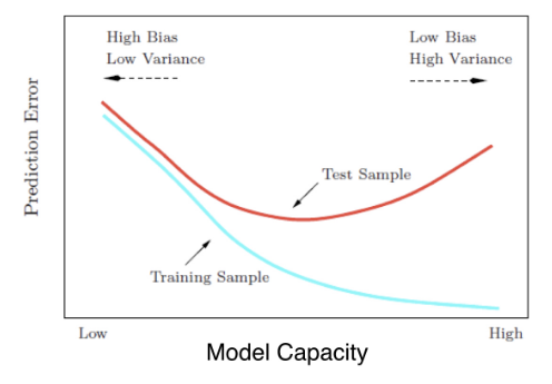
Thinking about model capacity

  • Overfitting of
  • Workflow for optimizing model capacity
    • Start with a small network
    • Gradually increase capacity
    • Keep increasing capacity until validation score is no longer improving

Stepping up to images

Building your own digit recognition model

You've reached the final exercise of the course - you now know everything you need to build an accurate model to recognize handwritten digits!

To add an extra challenge, we've loaded only 2500 images, rather than 60000 which you will see in some published results. Deep learning models perform better with more data, however, they also take longer to train, especially when they start becoming more complex.

If you have a computer with a CUDA compatible GPU, you can take advantage of it to improve computation time. If you don't have a GPU, no problem! You can set up a deep learning environment in the cloud that can run your models on a GPU. Here is a blog post by Dan that explains how to do this - check it out after completing this exercise! It is a great next step as you continue your deep learning journey.

mnist = pd.read_csv('./dataset/mnist.csv', header=None)
mnist.head()
0 1 2 3 4 5 6 7 8 9 ... 775 776 777 778 779 780 781 782 783 784
0 5 0 0.1 0.2 0.3 0.4 0.5 0.6 0.7 0.8 ... 0.608 0.609 0.61 0.611 0.612 0.613 0.614 0.615 0.616 0.617
1 4 0 0.0 0.0 0.0 0.0 0.0 0.0 0.0 0.0 ... 0.000 0.000 0.00 0.000 0.000 0.000 0.000 0.000 0.000 0.000
2 3 0 0.0 0.0 0.0 0.0 0.0 0.0 0.0 0.0 ... 0.000 0.000 0.00 0.000 0.000 0.000 0.000 0.000 0.000 0.000
3 0 0 0.0 0.0 0.0 0.0 0.0 0.0 0.0 0.0 ... 0.000 0.000 0.00 0.000 0.000 0.000 0.000 0.000 0.000 0.000
4 2 0 0.0 0.0 0.0 0.0 0.0 0.0 0.0 0.0 ... 0.000 0.000 0.00 0.000 0.000 0.000 0.000 0.000 0.000 0.000

5 rows × 785 columns

X = mnist.iloc[:, 1:].astype(np.float32).to_numpy()
y = to_categorical(mnist.iloc[:, 0])
model = tf.keras.Sequential()

# Add the first hidden layer
model.add(tf.keras.layers.Dense(50, activation='relu', input_shape=(X.shape[1], )))

# Add the second hidden layer
model.add(tf.keras.layers.Dense(50, activation='relu'))

# Add the output layer
model.add(tf.keras.layers.Dense(10, activation='softmax'))

# Compile the model
model.compile(optimizer='adam', loss='categorical_crossentropy', metrics=['accuracy'])

# Fit the model
model.fit(X, y, validation_split=0.3, epochs=50);
Epoch 1/50
44/44 [==============================] - 0s 3ms/step - loss: 18.8407 - accuracy: 0.4229 - val_loss: 7.5732 - val_accuracy: 0.5391
Epoch 2/50
44/44 [==============================] - 0s 2ms/step - loss: 4.0665 - accuracy: 0.6879 - val_loss: 4.7740 - val_accuracy: 0.6456
Epoch 3/50
44/44 [==============================] - 0s 2ms/step - loss: 2.1160 - accuracy: 0.7729 - val_loss: 4.4106 - val_accuracy: 0.6689
Epoch 4/50
44/44 [==============================] - 0s 2ms/step - loss: 1.2134 - accuracy: 0.8307 - val_loss: 3.7577 - val_accuracy: 0.6839
Epoch 5/50
44/44 [==============================] - 0s 2ms/step - loss: 0.9683 - accuracy: 0.8614 - val_loss: 3.5194 - val_accuracy: 0.7238
Epoch 6/50
44/44 [==============================] - 0s 2ms/step - loss: 0.5479 - accuracy: 0.9114 - val_loss: 3.1736 - val_accuracy: 0.7288
Epoch 7/50
44/44 [==============================] - 0s 2ms/step - loss: 0.3776 - accuracy: 0.9221 - val_loss: 3.3420 - val_accuracy: 0.7255
Epoch 8/50
44/44 [==============================] - 0s 2ms/step - loss: 0.2887 - accuracy: 0.9329 - val_loss: 3.0673 - val_accuracy: 0.7338
Epoch 9/50
44/44 [==============================] - 0s 2ms/step - loss: 0.1504 - accuracy: 0.9664 - val_loss: 3.0627 - val_accuracy: 0.7371
Epoch 10/50
44/44 [==============================] - 0s 2ms/step - loss: 0.0817 - accuracy: 0.9800 - val_loss: 3.0174 - val_accuracy: 0.7438
Epoch 11/50
44/44 [==============================] - 0s 2ms/step - loss: 0.0606 - accuracy: 0.9821 - val_loss: 3.0648 - val_accuracy: 0.7388
Epoch 12/50
44/44 [==============================] - 0s 2ms/step - loss: 0.0328 - accuracy: 0.9879 - val_loss: 3.0618 - val_accuracy: 0.7537
Epoch 13/50
44/44 [==============================] - 0s 2ms/step - loss: 0.0253 - accuracy: 0.9914 - val_loss: 2.9957 - val_accuracy: 0.7687
Epoch 14/50
44/44 [==============================] - 0s 2ms/step - loss: 0.0132 - accuracy: 0.9964 - val_loss: 3.0766 - val_accuracy: 0.7521
Epoch 15/50
44/44 [==============================] - 0s 2ms/step - loss: 0.0045 - accuracy: 0.9993 - val_loss: 3.0787 - val_accuracy: 0.7471
Epoch 16/50
44/44 [==============================] - 0s 2ms/step - loss: 0.0019 - accuracy: 1.0000 - val_loss: 3.0682 - val_accuracy: 0.7537
Epoch 17/50
44/44 [==============================] - 0s 2ms/step - loss: 0.0017 - accuracy: 1.0000 - val_loss: 3.0551 - val_accuracy: 0.7554
Epoch 18/50
44/44 [==============================] - 0s 2ms/step - loss: 9.4450e-04 - accuracy: 1.0000 - val_loss: 3.0612 - val_accuracy: 0.7504
Epoch 19/50
44/44 [==============================] - 0s 2ms/step - loss: 7.6430e-04 - accuracy: 1.0000 - val_loss: 3.0624 - val_accuracy: 0.7504
Epoch 20/50
44/44 [==============================] - 0s 2ms/step - loss: 6.7846e-04 - accuracy: 1.0000 - val_loss: 3.0623 - val_accuracy: 0.7521
Epoch 21/50
44/44 [==============================] - 0s 2ms/step - loss: 6.2465e-04 - accuracy: 1.0000 - val_loss: 3.0610 - val_accuracy: 0.7537
Epoch 22/50
44/44 [==============================] - 0s 2ms/step - loss: 5.8118e-04 - accuracy: 1.0000 - val_loss: 3.0643 - val_accuracy: 0.7504
Epoch 23/50
44/44 [==============================] - 0s 2ms/step - loss: 5.3415e-04 - accuracy: 1.0000 - val_loss: 3.0627 - val_accuracy: 0.7537
Epoch 24/50
44/44 [==============================] - 0s 2ms/step - loss: 5.0316e-04 - accuracy: 1.0000 - val_loss: 3.0637 - val_accuracy: 0.7537
Epoch 25/50
44/44 [==============================] - 0s 2ms/step - loss: 4.6953e-04 - accuracy: 1.0000 - val_loss: 3.0648 - val_accuracy: 0.7537
Epoch 26/50
44/44 [==============================] - 0s 2ms/step - loss: 4.3986e-04 - accuracy: 1.0000 - val_loss: 3.0635 - val_accuracy: 0.7537
Epoch 27/50
44/44 [==============================] - 0s 2ms/step - loss: 4.1727e-04 - accuracy: 1.0000 - val_loss: 3.0630 - val_accuracy: 0.7537
Epoch 28/50
44/44 [==============================] - 0s 2ms/step - loss: 3.9517e-04 - accuracy: 1.0000 - val_loss: 3.0641 - val_accuracy: 0.7537
Epoch 29/50
44/44 [==============================] - 0s 2ms/step - loss: 3.7410e-04 - accuracy: 1.0000 - val_loss: 3.0674 - val_accuracy: 0.7537
Epoch 30/50
44/44 [==============================] - 0s 2ms/step - loss: 3.5648e-04 - accuracy: 1.0000 - val_loss: 3.0671 - val_accuracy: 0.7554
Epoch 31/50
44/44 [==============================] - 0s 2ms/step - loss: 3.3969e-04 - accuracy: 1.0000 - val_loss: 3.0688 - val_accuracy: 0.7554
Epoch 32/50
44/44 [==============================] - 0s 2ms/step - loss: 3.2434e-04 - accuracy: 1.0000 - val_loss: 3.0653 - val_accuracy: 0.7554
Epoch 33/50
44/44 [==============================] - 0s 2ms/step - loss: 3.1208e-04 - accuracy: 1.0000 - val_loss: 3.0667 - val_accuracy: 0.7554
Epoch 34/50
44/44 [==============================] - 0s 2ms/step - loss: 2.9868e-04 - accuracy: 1.0000 - val_loss: 3.0664 - val_accuracy: 0.7554
Epoch 35/50
44/44 [==============================] - 0s 2ms/step - loss: 2.8480e-04 - accuracy: 1.0000 - val_loss: 3.0667 - val_accuracy: 0.7554
Epoch 36/50
44/44 [==============================] - 0s 2ms/step - loss: 2.7411e-04 - accuracy: 1.0000 - val_loss: 3.0662 - val_accuracy: 0.7554
Epoch 37/50
44/44 [==============================] - 0s 6ms/step - loss: 2.6219e-04 - accuracy: 1.0000 - val_loss: 3.0684 - val_accuracy: 0.7537
Epoch 38/50
44/44 [==============================] - 0s 2ms/step - loss: 2.5434e-04 - accuracy: 1.0000 - val_loss: 3.0676 - val_accuracy: 0.7554
Epoch 39/50
44/44 [==============================] - 0s 2ms/step - loss: 2.4130e-04 - accuracy: 1.0000 - val_loss: 3.0685 - val_accuracy: 0.7537
Epoch 40/50
44/44 [==============================] - 0s 2ms/step - loss: 2.3264e-04 - accuracy: 1.0000 - val_loss: 3.0675 - val_accuracy: 0.7554
Epoch 41/50
44/44 [==============================] - 0s 2ms/step - loss: 2.2436e-04 - accuracy: 1.0000 - val_loss: 3.0682 - val_accuracy: 0.7554
Epoch 42/50
44/44 [==============================] - 0s 2ms/step - loss: 2.1692e-04 - accuracy: 1.0000 - val_loss: 3.0698 - val_accuracy: 0.7537
Epoch 43/50
44/44 [==============================] - 0s 2ms/step - loss: 2.0934e-04 - accuracy: 1.0000 - val_loss: 3.0683 - val_accuracy: 0.7554
Epoch 44/50
44/44 [==============================] - 0s 2ms/step - loss: 2.0208e-04 - accuracy: 1.0000 - val_loss: 3.0703 - val_accuracy: 0.7554
Epoch 45/50
44/44 [==============================] - 0s 2ms/step - loss: 1.9523e-04 - accuracy: 1.0000 - val_loss: 3.0680 - val_accuracy: 0.7554
Epoch 46/50
44/44 [==============================] - 0s 2ms/step - loss: 1.8736e-04 - accuracy: 1.0000 - val_loss: 3.0668 - val_accuracy: 0.7571
Epoch 47/50
44/44 [==============================] - 0s 2ms/step - loss: 1.7953e-04 - accuracy: 1.0000 - val_loss: 3.0687 - val_accuracy: 0.7554
Epoch 48/50
44/44 [==============================] - 0s 2ms/step - loss: 1.7335e-04 - accuracy: 1.0000 - val_loss: 3.0697 - val_accuracy: 0.7554
Epoch 49/50
44/44 [==============================] - 0s 2ms/step - loss: 1.6714e-04 - accuracy: 1.0000 - val_loss: 3.0696 - val_accuracy: 0.7571
Epoch 50/50
44/44 [==============================] - 0s 2ms/step - loss: 1.6202e-04 - accuracy: 1.0000 - val_loss: 3.0690 - val_accuracy: 0.7571