Masks and Filters in Biomedical Image Analysis
Cut image processing to the bone by transforming x-ray images. You'll learn how to exploit intensity patterns to select sub-regions of an array, and you'll use convolutional filters to detect interesting features. You'll also use SciPy's ndimage module, which contains a treasure trove of image processing tools. This is the Summary of lecture "Biomedical Image Analysis in Python", via datacamp.


import numpy as np
import matplotlib.pyplot as plt
import imageio

plt.rcParams['figure.figsize'] = (10, 8)
Intensity
In this chapter, we will work with a hand radiograph from a 2017 Radiological Society of North America competition. X-ray absorption is highest in dense tissue such as bone, so the resulting intensities should be high. Consequently, images like this can be used to predict "bone age" in children.
To start, let's load the image and check its intensity range.
The image datatype determines the range of possible intensities: e.g., 8-bit unsigned integers (uint8) can take values in the range of 0 to 255. A colorbar can be helpful for connecting these values to the visualized image.
def format_and_render_plot():
    '''Custom function to simplify common formatting operations for exercises. Operations include:
    1. Turning off axis grids.
    2. Calling `plt.tight_layout` to improve subplot spacing.
    3. Calling `plt.show()` to render plot.'''
    fig = plt.gcf()
    for ax in fig.axes:
        ax.axis('off')
    plt.tight_layout()
    plt.show()
im = imageio.imread('./dataset/hand.png')
im = im.astype('float64')
print('Data type:', im.dtype)
print('Min value:', im.min())
print('Max value:', im.max())

# Plot the grayscale image
plt.imshow(im, cmap='gray', vmin=0, vmax=255);
plt.colorbar();

Histograms
Histograms display the distribution of values in your image by binning each element by its intensity then measuring the size of each bin.
The area under a histogram is called the cumulative distribution function (CDF for short). It measures the frequency with which a given range of pixel intensities occurs.
For this exercise, describe the intensity distribution in im by calculating the histogram and cumulative distribution function and displaying them together.
def format_and_render_plot():
    '''Custom function to simplify common formatting operations for exercises. Operations include:
    1. Turning off axis grids.
    2. Calling `plt.tight_layout` to improve subplot spacing.
    3. Calling `plt.show()` to render plot.'''
    fig = plt.gcf()
    for ax in fig.axes:
        ax.legend(loc='center right')
    plt.show()
import scipy.ndimage as ndi

# Create a histogram, binned at each possible value
hist = ndi.histogram(im, min=0, max=255, bins=256)

# Create a cumulative distribution function
cdf = hist.cumsum() / hist.sum()

# Plot the histogram and CDF
fig, axes = plt.subplots(2, 1, sharex=True)
axes[0].plot(hist, label='Histogram');
axes[1].plot(cdf, label='CDF');
format_and_render_plot();

You can see the data is clumped into a few separate distributions, consisting of background noise, skin, bone, and artifacts. Sometimes we can separate these well with global thresholds (foreground/background); other times the distributions overlap quite a bit (skin/bone).
Create a mask
Masks are the primary method for removing or selecting specific parts of an image. They are binary arrays that indicate whether a value should be included in an analysis. Typically, masks are created by applying one or more logical operations to an image.
For this exercise, try to use a simple intensity threshold to differentiate between skin and bone in the hand radiograph.
def format_and_render_plot():
    '''Custom function to simplify common formatting operations for exercises. Operations include:
    1. Turning off axis grids.
    2. Calling `plt.tight_layout` to improve subplot spacing.
    3. Calling `plt.show()` to render plot.'''
    fig = plt.gcf()
    for ax in fig.axes:
        ax.axis('off')
    plt.tight_layout()
    plt.show()
mask_bone = im >= 75
mask_skin = (im >= 35) & (im < 75)

# Plot the skin (0) and bone (1) masks
fig, axes = plt.subplots(1, 2)
axes[0].imshow(mask_skin, cmap='gray')
axes[1].imshow(mask_bone, cmap='gray')
format_and_render_plot()

Apply a mask
Although masks are binary, they can be applied to images to filter out pixels where the mask is False.
NumPy's where() function is a flexible way of applying masks. It takes three arguments:
np.where(condition, x, y)
condition, x and y can be either arrays or single values. This allows you to pass through original image values while setting masked values to 0.
Let's practice applying masks by selecting the bone-like pixels from the hand x-ray (im).
def format_and_render_plot():
    '''Custom function to simplify common formatting operations for exercises. Operations include:
    1. Turning off axis grids.
    2. Calling `plt.tight_layout` to improve subplot spacing.
    3. Calling `plt.show()` to render plot.'''
    fig = plt.gcf()
    fig.axes[0].axis('off')
    plt.tight_layout()
    plt.show()
mask_bone = im >= 75
im_bone = np.where(mask_bone, im, 0)

# Get the histogram of bone intensity
hist = ndi.histogram(im_bone, min=1, max=255, bins=255)

# Plot masked image and histogram
fig, axes = plt.subplots(2, 1)
axes[0].imshow(im_bone, cmap='gray')
axes[1].plot(hist)
format_and_render_plot()

Tune a mask
Imperfect masks can be tuned through the addition and subtraction of pixels. SciPy includes several useful methods for accomplishing these ends. These include:
-
binary_dilation: Add pixels along edges -
binary_erosion: Remove pixels along edges -
binary_opening: Erode then dilate, "opening" areas near edges -
binary_closing: Dilate then erode, "filling in" holes
For this exercise, create a bone mask then tune it to include additional pixels.
mask_bone = im >= 75
mask_dilate = ndi.binary_dilation(mask_bone, iterations=5)
mask_closed = ndi.binary_closing(mask_bone, iterations=5)

# Plot masked images
fig, axes = plt.subplots(1, 3)
axes[0].imshow(mask_bone, cmap='gray')
axes[1].imshow(mask_dilate, cmap='gray')
axes[2].imshow(mask_closed, cmap='gray')
format_and_render_plot()

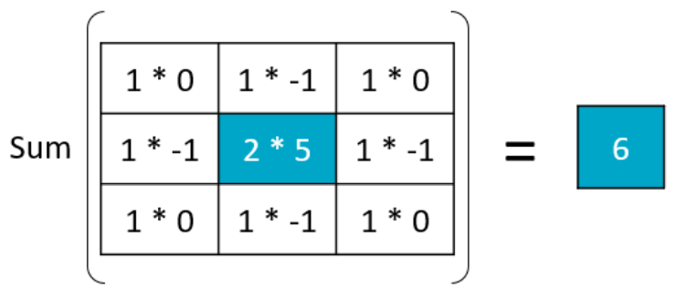
Filter convolutions
Filters are an essential tool in image processing. They allow you to transform images based on intensity values surrounding a pixel, rather than globally.
For this exercise, smooth the foot radiograph. First, specify the weights to be used. (These are called "footprints" and "kernels" as well.) Then, convolve the filter with im and plot the result.
def format_and_render_plot():
    '''Custom function to simplify common formatting operations for exercises. Operations include:
    1. Turning off axis grids.
    2. Calling `plt.tight_layout` to improve subplot spacing.
    3. Calling `plt.show()` to render plot.'''
    fig = plt.gcf()
    for ax in fig.axes:
        ax.axis('off')
    plt.tight_layout()
    plt.show()
weights = [[0.11, 0.11, 0.11],
           [0.11, 0.11, 0.11],
           [0.11, 0.11, 0.11]]

# Convolve the image with the filter
im_filt = ndi.convolve(im, weights)

# Plot the images
fig, axes = plt.subplots(1, 2)
axes[0].imshow(im, cmap='gray')
axes[1].imshow(im_filt, cmap='gray')
format_and_render_plot()

Smoothing
Smoothing can improve the signal-to-noise ratio(SNR for short) of your image by blurring out small variations in intensity. The Gaussian filter is excellent for this: it is a circular (or spherical) smoothing kernel that weights nearby pixels higher than distant ones.
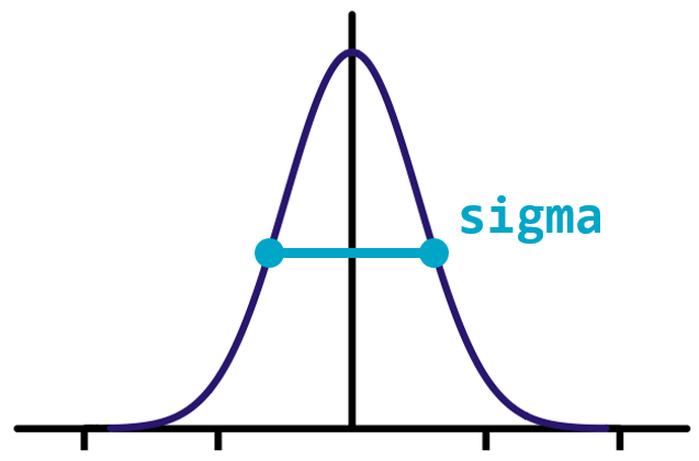
The width of the distribution is controlled by the sigma argument, with higher values leading to larger smoothing effects.
For this exercise, test the effects of applying Gaussian filters to the foot x-ray before creating a bone mask.
im_s1 = ndi.gaussian_filter(im, sigma=1)
im_s3 = ndi.gaussian_filter(im, sigma=3)

# Draw bone masks of each image
fig, axes = plt.subplots(1, 3)
axes[0].imshow(im >= 75, cmap='gray')
axes[1].imshow(im_s1 >= 75, cmap='gray')
axes[2].imshow(im_s3 >= 75, cmap='gray')
format_and_render_plot()

Detect edges (1)
Filters can also be used as "detectors." If a part of the image fits the weighting pattern, the returned value will be very high (or very low).
In the case of edge detection, that pattern is a change in intensity along a plane. A filter detecting horizontal edges might look like this:
weights = [[+1, +1, +1],
           [ 0,  0,  0],
           [-1, -1, -1]]
For this exercise, create a vertical edge detector and see how well it performs on the hand x-ray (im).
weights = [[1, 0, -1], [1, 0, -1], [1, 0, -1]]

# Convolve "im" with filter weights
edges = ndi.convolve(im, weights)

# Draw the image in color
plt.imshow(edges, cmap='seismic', vmin=-75, vmax=75);
plt.colorbar();
format_and_render_plot();

Detect edges (2)
Edge detection can be performed along multiple axes, then combined into a single edge value. For 2D images, the horizontal and vertical "edge maps" can be combined using the Pythagorean theorem:
$$ z = \sqrt{x^2 + y^2} $$
One popular edge detector is the Sobel filter. The Sobel filter provides extra weight to the center pixels of the detector:
weights = [[ 1,  2,  1],
           [ 0,  0,  0],
           [-1, -2, -1]]
For this exercise, improve upon your previous detection effort by merging the results of two Sobel-filtered images into a composite edge map.
def format_and_render_plot():
    '''Custom function to simplify common formatting operations for exercises. Operations include:
    1. Turning off axis grids.
    2. Calling `plt.tight_layout` to improve subplot spacing.
    3. Calling `plt.show()` to render plot.'''
    fig = plt.gcf()
    fig.axes[0].axis('off')
    plt.show()
sobel_ax0 = ndi.sobel(im, axis=0)
sobel_ax1 = ndi.sobel(im, axis=1)

# Calculate edge magnitude
edges = np.sqrt(np.square(sobel_ax0) + np.square(sobel_ax1))
plt.imshow(edges, cmap='gray', vmax=75)
format_and_render_plot()
