CNN with MNIST dataset
In this post, we will implement various type of CNN for MNIST dataset. In Tensorflow, there are various ways to define CNN model like sequential model, functional model, and sub-class model. We'll simply implement each type and test it.


- CNN model with sequential API
- Build model with Functional API
- Build model with Model Subclassing
- Build model with Model Ensemble
- Best CNN model in MNIST dataset
- Summary
import tensorflow as tf
import numpy as np
import matplotlib.pyplot as plt
import pandas as pd

plt.rcParams['figure.figsize'] = (16, 10)
plt.rc('font', size=15)
CNN model with sequential API
Previously, we learned basic operation of convolution and max-pooling. Actually, we already implemented simple type of CNN model for MNIST classification, which is manually combined with 2D convolution layer and max-pooling layer. But there are other ways to define CNN model. In this section, we will implement CNN model with Sequential API.
Briefly speaking, we will build the model as follows,
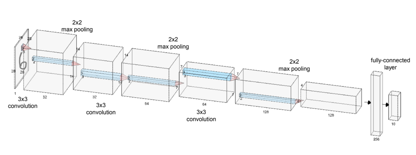
3x3 2D convolution layer is defined as an input layer, and post-process with 2x2 max-pooling. And these process will be redundant 3 times, then set fully-connected layer as an output layer for classification. In convolution layer, stride will be 1, and padding will be same (that is, we will use half padding). And in max-pooling layer, stride will be 2, and padding will also be same.
learning_rate = 0.001
training_epochs = 15
batch_size = 100
And for the tracking model training, it is helpful to build checkpoint while training the model, so when we the model training is failed due to unexpected reason, we can re-train it with checkpoint.
import os

cur_dir = os.getcwd()
checkpoint_dir = os.path.join(cur_dir, 'checkpoints', 'mnist_cnn_seq')
os.makedirs(checkpoint_dir, exist_ok=True)
checkpoint_prefix = os.path.join(checkpoint_dir, 'mnist_cnn_seq')
Data Pipelining
Before model implementation, it requires data pipelining, also known as data-preprocess. As you can see from previous example, the original raw data is hardly used directly. So we need to normalize it, convert it, that we can express whole process as an "data-preprocessing".
Note that, the label of each data is class label. So to use it in Neural network model, it needs to encode it as an binary code. Maybe someone already knew it, it is one-hot encoding. Luckily, tf.keras also implements to_categorical for one-hot encoding.
from tensorflow.keras.utils import to_categorical

# MNIST dataset
(X_train, y_train), (X_test, y_test) = tf.keras.datasets.mnist.load_data()

# Normalization
X_train = X_train.astype(np.float32) / 255.
X_test = X_test.astype(np.float32) / 255.

# Convert it to 4D array (or we can use np.expand_dims for dimension expansion)
X_train = X_train[..., tf.newaxis]
X_test = X_test[..., tf.newaxis]

# one-hot encoding
y_train = to_categorical(y_train, 10)
y_test = to_categorical(y_test, 10)

# Build dataset pipeline
train_ds = tf.data.Dataset.from_tensor_slices((X_train, y_train)).shuffle(buffer_size=100000).batch(batch_size)
test_ds = tf.data.Dataset.from_tensor_slices((X_test, y_test)).batch(batch_size)
def create_model():
    model = tf.keras.Sequential(name='CNN_Sequential')
    model.add(tf.keras.layers.Conv2D(filters=32, kernel_size=(3, 3), activation=tf.keras.activations.relu,
                                     padding='SAME', input_shape=(28, 28, 1)))
    model.add(tf.keras.layers.MaxPool2D(padding='SAME'))
    model.add(tf.keras.layers.Conv2D(filters=64, kernel_size=(3, 3), activation=tf.keras.activations.relu,
                                     padding='SAME'))
    model.add(tf.keras.layers.MaxPool2D(padding='SAME'))
    model.add(tf.keras.layers.Conv2D(filters=128, kernel_size=(3, 3), activation=tf.keras.activations.relu,
                                     padding='SAME'))
    model.add(tf.keras.layers.MaxPool2D(padding='SAME'))
    model.add(tf.keras.layers.Flatten())
    model.add(tf.keras.layers.Dense(256, activation=tf.keras.activations.relu))
    model.add(tf.keras.layers.Dropout(0.4))
    model.add(tf.keras.layers.Dense(10))
    return model

# Create model
model = create_model()
model.summary()
Note that, when we directly add the layer, we need to enter the input data for generating output. But in Sequential model, each previous layers node is connected with next layers node automatically, All we need to do is to input the data in the model, then output will be generated from the whole model.
def loss_fn(model, images, labels):
    logits = model(images, training=True)
    loss = tf.reduce_mean(tf.nn.softmax_cross_entropy_with_logits(logits=logits, labels=labels))
    return loss

# Gradient Function
def grad(model, images, labels):
    with tf.GradientTape() as tape:
        loss = loss_fn(model, images, labels)
    return tape.gradient(loss, model.trainable_variables)
Optimizer and Evaluation
For finding optimum value, we will use "Adam" Optimizer with predifined learning_rate. Also, we need to define evaluation function so that we can check the performance (or accuracy of model).
One more thing, We already mention that checkpoint is required for tracking history. So we will define it here.
optimizer = tf.keras.optimizers.Adam(learning_rate=learning_rate)

# Evaluation function
def evaluate(model, images, labels):
    logits = model(images, training=False)
    correct_predict = tf.equal(tf.argmax(logits, 1), tf.argmax(labels, 1))
    accuracy = tf.reduce_mean(tf.cast(correct_predict, tf.float32))
    return accuracy

# Checkpoint
checkpoint = tf.train.Checkpoint(cnn=model)
for e in range(training_epochs):
    avg_loss = 0.
    avg_train_acc = 0.
    avg_test_acc = 0.
    train_step = 0
    test_step = 0

    for images, labels in train_ds:
        grads = grad(model, images, labels)
        optimizer.apply_gradients(zip(grads, model.trainable_variables))
        loss = loss_fn(model, images, labels)
        acc = evaluate(model, images, labels)
        avg_loss = avg_loss + loss
        avg_train_acc = avg_train_acc + acc
        train_step += 1
    avg_loss = avg_loss / train_step
    avg_train_acc = avg_train_acc / train_step

    for images, labels in test_ds:
        acc = evaluate(model, images, labels)
        avg_test_acc = avg_test_acc + acc
        test_step += 1
    avg_test_acc = avg_test_acc / test_step

    print("Epoch: {}".format(e + 1),
          "loss: {:.8f}".format(avg_loss),
          "train acc: {:.4f}".format(avg_train_acc),
          "test acc: {:.4f}".format(avg_test_acc))

    checkpoint.save(file_prefix=checkpoint_prefix)
Build model with Functional API
We can find out that it works in Sequential API. Now let's implement it with another approach, the Functional APIs. Whole process will be same, except building model section.
There is some limitation while building model with Sequential API. As you can see from create_model, whole layers are connected in one pipeline. But what if we want to use multi-input, or multi-output? And in Sequaltial API, we cannot mannually build the layer block. For instance, ResNet uses specific block named residual block that contained skip connection. But we cannot implement manual block in sequential API. Or we cannot build shared layers, so same layer is called several times.
Actually, building process is almost similar with that of Sequential API. All we need to do is to define input, output, and connect each layers like this,
def create_model_functional():
    inputs = tf.keras.Input(shape=(28, 28, 1))
    conv1 = tf.keras.layers.Conv2D(filters=32, kernel_size=(3, 3), padding='SAME',
                                   activation=tf.keras.activations.relu)(inputs)
    pool1 = tf.keras.layers.MaxPool2D(padding='SAME')(conv1)
    conv2 = tf.keras.layers.Conv2D(filters=64, kernel_size=(3, 3), padding='SAME',
                                   activation=tf.keras.activations.relu)(pool1)
    pool2 = tf.keras.layers.MaxPool2D(padding='SAME')(conv2)
    conv3 = tf.keras.layers.Conv2D(filters=128, kernel_size=(3, 3), padding='SAME',
                                   activation=tf.keras.activations.relu)(pool2)
    pool3 = tf.keras.layers.MaxPool2D(padding='SAME')(conv3)
    pool3_flat = tf.keras.layers.Flatten()(pool3)
    dense4 = tf.keras.layers.Dense(units=256, activation=tf.keras.activations.relu)(pool3_flat)
    drop4 = tf.keras.layers.Dropout(rate=0.4)(dense4)
    logits = tf.keras.layers.Dense(units=10)(drop4)
    return tf.keras.Model(inputs=inputs, outputs=logits)
model = create_model_functional()
model.summary()
As you can see the summary of model, the total parameter is the same as previous one. Interest thing is that the default name is defined as "functional_x". From these, we can found out that our new model is implemented with functional API.
One more example, in Residual block, we can implement skip connection like this,
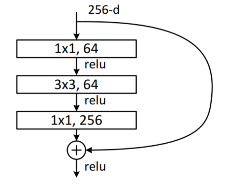
inputs = tf.keras.Input(shape=(28, 28, 256))
conv1 = tf.keras.layers.Conv2D(filters=64, kernel_size=(1, 1), padding='SAME', activation=tf.keras.activations.relu)(inputs)
conv2 = tf.keras.layers.Conv2D(filters=64, kernel_size=(3, 3), padding='SAME', activation=tf.keras.activations.relu)(conv1)
conv3 = tf.keras.layers.Conv2D(filters=256, kernel_size=(1, 1), padding='SAME')(conv2)
# skip connection
add3 = tf.keras.layers.add([conv3, inputs])
relu3 = tf.keras.activations.relu(add3)
model = tf.keras.Model(inputs=inputs, outputs=relu3)
Build model with Model Subclassing
The other way to build model is Subclassing. Technically, it is defined model with python Class. Model Subclassing is the approach to build a fully-customizable model by subclassing tf.keras.Model. So we can define the inital implementation like layer, node parameter on __init__ method, and forward pass on call method.
class CNNModel(tf.keras.Model):
    def __init__(self):
        super(CNNModel, self).__init__()
        self.conv1 = tf.keras.layers.Conv2D(filters=32, kernel_size=(3, 3), padding='SAME',
                                            activation=tf.keras.activations.relu)
        self.pool1 = tf.keras.layers.MaxPool2D(padding='SAME')
        self.conv2 = tf.keras.layers.Conv2D(filters=64, kernel_size=(3, 3), padding='SAME',
                                            activation=tf.keras.activations.relu)
        self.pool2 = tf.keras.layers.MaxPool2D(padding='SAME')
        self.conv3 = tf.keras.layers.Conv2D(filters=128, kernel_size=(3, 3), padding='SAME',
                                            activation=tf.keras.activations.relu)
        self.pool3 = tf.keras.layers.MaxPool2D(padding='SAME')
        self.pool3_flat = tf.keras.layers.Flatten()
        self.dense4 = tf.keras.layers.Dense(units=256, activation=tf.keras.activations.relu)
        self.drop4 = tf.keras.layers.Dropout(rate=0.4)
        self.dense5 = tf.keras.layers.Dense(units=10)

    def call(self, inputs, training=False):
        net = self.conv1(inputs)
        net = self.pool1(net)
        net = self.conv2(net)
        net = self.pool2(net)
        net = self.conv3(net)
        net = self.pool3(net)
        net = self.pool3_flat(net)
        net = self.dense4(net)
        net = self.drop4(net)
        net = self.dense5(net)
        return net
model = CNNModel()
Actually, we just instantiate the CNNModel class, so the connection is not connected when instantiates. If we want to find the summary of this network, we need to build it or fit it with some data.
model.build(input_shape=(1, 28, 28, 1))
model.summary()
Same as before model.
Build model with Model Ensemble
The last method to build model is Ensemble method. Actually, the keyword ensemble is from statistics and machine learning. In wikipedia, it is defined that this method use multiple learning algorithms to obtain better predictive performance than could be obtained from any of the constituent learning algorithm alone. If you know about the Machine Learning, Random Forest is an ensemble model using bagging approach.
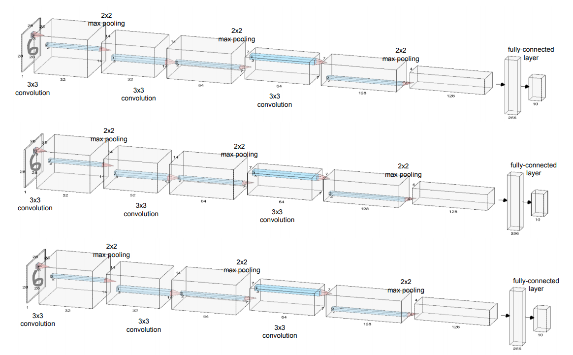
In short, we can run several CNN Networks simultaneously, and choose the best network that shows good performance.
At the first step, we build the base model with Model Subclassing.
class CNNModel(tf.keras.Model):
    def __init__(self):
        super(CNNModel, self).__init__()
        self.conv1 = tf.keras.layers.Conv2D(filters=32, kernel_size=(3, 3), padding='SAME',
                                            activation=tf.keras.activations.relu)
        self.pool1 = tf.keras.layers.MaxPool2D(padding='SAME')
        self.conv2 = tf.keras.layers.Conv2D(filters=64, kernel_size=(3, 3), padding='SAME',
                                            activation=tf.keras.activations.relu)
        self.pool2 = tf.keras.layers.MaxPool2D(padding='SAME')
        self.conv3 = tf.keras.layers.Conv2D(filters=128, kernel_size=(3, 3), padding='SAME',
                                            activation=tf.keras.activations.relu)
        self.pool3 = tf.keras.layers.MaxPool2D(padding='SAME')
        self.pool3_flat = tf.keras.layers.Flatten()
        self.dense4 = tf.keras.layers.Dense(units=256, activation=tf.keras.activations.relu)
        self.drop4 = tf.keras.layers.Dropout(rate=0.4)
        self.dense5 = tf.keras.layers.Dense(units=10)

    def call(self, inputs, training=False):
        net = self.conv1(inputs)
        net = self.pool1(net)
        net = self.conv2(net)
        net = self.pool2(net)
        net = self.conv3(net)
        net = self.pool3(net)
        net = self.pool3_flat(net)
        net = self.dense4(net)
        net = self.drop4(net)
        net = self.dense5(net)
        return net
Now, here is the point. If we want use 3 models for ensemble, we just instantiate each model and append it to the list like this,
models = []
for m in range(3):
    models.append(CNNModel())
We can use same loss and gradient function as previous, since all function is focused on one model. But our purpose is choose the best model of test dataset, so we need to change evaluate method for multiple models. Also, we need to modify checkpoint saving.
def loss_fn(model, images, labels):
    logits = model(images, training=True)
    loss = tf.reduce_mean(tf.nn.softmax_cross_entropy_with_logits(logits=logits, labels=labels))
    return loss

# Gradient Function
def grad(model, images, labels):
    with tf.GradientTape() as tape:
        loss = loss_fn(model, images, labels)
    return tape.gradient(loss, model.trainable_variables)
optimizer = tf.keras.optimizers.Adam(learning_rate=learning_rate)

def evaluate(models, images, labels):
    predicts = tf.zeros_like(labels)
    for model in models:
        logits = model(images, training=False)
        predicts += logits
    correct_predict = tf.equal(tf.argmax(predicts, 1), tf.argmax(labels, 1))
    accuracy = tf.reduce_mean(tf.cast(correct_predict, tf.float32))
    return accuracy

checkpoints = []
for model in models:
    checkpoints.append(tf.train.Checkpoint(cnn=model))
And, of course, training and validation process will be changed for multiple models.
for e in range(training_epochs):
    avg_loss = 0.
    avg_train_acc = 0.
    avg_test_acc = 0.
    train_step = 0
    test_step = 0

    for images, labels in train_ds:
        for model in models:
            grads = grad(model, images, labels)
            optimizer.apply_gradients(zip(grads, model.trainable_variables))
            loss = loss_fn(model, images, labels)
            avg_loss += loss / 3
        acc = evaluate(models, images, labels)
        avg_train_acc += acc
        train_step += 1
    avg_loss = avg_loss / train_step
    avg_train_acc = avg_train_acc / train_step

    for images, labels in test_ds:
        acc = evaluate(models, images, labels)
        avg_test_acc += acc
        test_step += 1
    avg_test_acc = avg_test_acc / test_step

    print("Epoch: {}".format(e + 1),
          "Loss: {:.8f}".format(avg_loss),
          "Train Accuracy: {:.4f}".format(avg_train_acc),
          "Test Accuracy: {:.4f}".format(avg_test_acc))

    for idx, checkpoint in enumerate(checkpoints):
        checkpoint.save(file_prefix=checkpoint_prefix+'-{}'.format(idx))
Initial accuracy is already high in 99%, we cannot check improvement of ensemble method, but if you stuck in low performance on inference, we maybe apply this kind of approach.
Best CNN model in MNIST dataset
We covered various type of model implementation, and also introduced ensemble method for model improvement. But there are other ways to improve model performance.
Actually, while we modify the network model, we may be faced with the Overfitting/Underfitting problem. This kind of problem is also known as Bias-Variance Tradeoff. The ultimate solution (if possible) for handling this is to add more data representing various patterns. But in real case, limitation of data amount is commonly occurred. So easiest way to increase data amount is regenerate the data from original data. Not only increasing the amount, we can also transform the image like rotation, color distribution, shift and so on. This approach is called Data Augmentation.
Data Augmentation
For image transformation, we use ndimage from scipy. And here, we will apply rotation and shift transformation from original dataset.
from scipy import ndimage
import random

def data_augmentation(images, labels):
    aug_images = []
    aug_labels = []

    for image, label in zip(images, labels):
        aug_images.append(image)
        aug_labels.append(label)

        # Background image for filling empty pixel
        bg_value = np.median(image)
        for _ in range(4):
            # Rotation
            rot_image = ndimage.rotate(image, angle=random.randint(-15, 15),
                                       reshape=False, cval=bg_value)
            # Shift
            shift_image = ndimage.shift(rot_image, shift=np.random.randint(-2, 2, 2),
                                        cval=bg_value)

            aug_images.append(shift_image)
            aug_labels.append(label)
    aug_images = np.array(aug_images)
    aug_labels = np.array(aug_labels)
    return aug_images, aug_labels
So while data-preprocessing, we need to apply data augmentation for original dataset.
(X_train, y_train), (X_test, y_test) = tf.keras.datasets.mnist.load_data()
X_train, y_train = data_augmentation(X_train, y_train)

# Convert numpy float type and normalize it
X_train = X_train.astype(np.float32) / 255.
X_test = X_test.astype(np.float32) / 255.

# Convert it to 4D array (or we can use np.expand_dims for dimension expansion)
X_train = X_train[..., tf.newaxis]
X_test = X_test[..., tf.newaxis]

# one-hot encoding
y_train = to_categorical(y_train, 10)
y_test = to_categorical(y_test, 10)

# Build dataset pipeline
train_ds = tf.data.Dataset.from_tensor_slices((X_train, y_train)).shuffle(buffer_size=500000).batch(batch_size)
test_ds = tf.data.Dataset.from_tensor_slices((X_test, y_test)).batch(batch_size)
Batch Normalization
Batch normalization is another form of regularization that rescales the output of a layer to make sure that have mean 0 and standard deviation 1 (that is, normal distribution). This approach is known as helping model training. We can apply this in our network. In this case, we will specific layers containing 1 convolution layer with batch normalization. And we can also apply kernel initialization with "Xavier initialization". (check the detail in previous post for Xavier initialization)
class ConvBNRelu(tf.keras.Model):
    def __init__(self, filters, kernel_size=(3, 3), strides=1, padding='SAME'):
        super(ConvBNRelu, self).__init__()
        self.conv = tf.keras.layers.Conv2D(filters=filters, kernel_size=kernel_size,
                                           strides=strides, padding=padding,
                                           kernel_initializer='glorot_normal')
        self.bn = tf.keras.layers.BatchNormalization()

    def call(self, inputs, training=False):
        net = self.conv(inputs)
        net = self.bn(net)
        return tf.keras.activations.relu(net)

class DenseBNRelu(tf.keras.Model):
    def __init__(self, units):
        super(DenseBNRelu, self).__init__()
        self.dense = tf.keras.layers.Dense(units=units, kernel_initializer='glorot_normal')
        self.bn = tf.keras.layers.BatchNormalization()

    def call(self, inputs, training=False):
        net = self.dense(inputs)
        net = self.bn(net)
        return tf.keras.activations.relu(net)
Same as before, we can build our model.
class CNNModel(tf.keras.Model):
    def __init__(self):
        super(CNNModel, self).__init__()
        self.conv1 = ConvBNRelu(filters=32, kernel_size=(3, 3), padding='SAME')
        self.pool1 = tf.keras.layers.MaxPool2D(padding='SAME')
        self.conv2 = ConvBNRelu(filters=64, kernel_size=(3, 3), padding='SAME')
        self.pool2 = tf.keras.layers.MaxPool2D(padding='SAME')
        self.conv3 = ConvBNRelu(filters=128, kernel_size=(3, 3), padding='SAME')
        self.pool3 = tf.keras.layers.MaxPool2D(padding='SAME')
        self.pool3_flat = tf.keras.layers.Flatten()
        self.dense4 = DenseBNRelu(units=256)
        self.drop4 = tf.keras.layers.Dropout(rate=0.4)
        self.dense5 = tf.keras.layers.Dense(units=10, kernel_initializer='glorot_normal')

    def call(self, inputs, training=False):
        net = self.conv1(inputs)
        net = self.pool1(net)
        net = self.conv2(net)
        net = self.pool2(net)
        net = self.conv3(net)
        net = self.pool3(net)
        net = self.pool3_flat(net)
        net = self.dense4(net)
        net = self.drop4(net)
        return self.dense5(net)
Then we apply the ensemble method. In this case, we will use 5 models.
models = []
for _ in range(5):
    models.append(CNNModel())
Same in loss function and gradient function
def loss_fn(model, images, labels):
    logits = model(images, training=True)
    loss = tf.reduce_mean(tf.nn.softmax_cross_entropy_with_logits(logits=logits, labels=labels))
    return loss

# Gradient Function
def grad(model, images, labels):
    with tf.GradientTape() as tape:
        loss = loss_fn(model, images, labels)
    return tape.gradient(loss, model.trainable_variables)

# Evaluation Function
def evaluate(models, images, labels):
    predicts = tf.zeros_like(labels)
    for model in models:
        logits = model(images, training=False)
        predicts += logits
    correct_predict = tf.equal(tf.argmax(predicts, 1), tf.argmax(labels, 1))
    accuracy = tf.reduce_mean(tf.cast(correct_predict, tf.float32))
    return accuracy
Exponential Decay
When back-propagation is process while training the model, learning_rate is kind of step_size when the optimizer is moved for finding optimal solution. If we changed our learning rate in depend on time (some called decaying, annealing whatever), it will easily find the optimal solution. There are other ways for learning rate scheduler like InverseTimeDecay, PolynomialDecay, etc. Find out more in here
lr_decay = tf.keras.optimizers.schedules.ExponentialDecay(learning_rate,
                                          decay_steps=X_train.shape[0] / batch_size * 5 * 5,
                                          decay_rate=0.5,
                                          staircase=True)

# Optimizer with learning rate scheduler
optimizer = tf.keras.optimizers.Adam(learning_rate=lr_decay)

# Checkpoint
checkpoints = []
for model in models:
    checkpoints.append(tf.train.Checkpoint(cnn=model))
for e in range(training_epochs):
    avg_loss = 0.
    avg_train_acc = 0.
    avg_test_acc = 0.
    train_step = 0
    test_step = 0

    for images, labels in train_ds:
        for model in models:
            grads = grad(model, images, labels)
            optimizer.apply_gradients(zip(grads, model.trainable_variables))
            loss = loss_fn(model, images, labels)
            avg_loss += loss / 3
        acc = evaluate(models, images, labels)
        avg_train_acc += acc
        train_step += 1
    avg_loss = avg_loss / train_step
    avg_train_acc = avg_train_acc / train_step

    for images, labels in test_ds:
        acc = evaluate(models, images, labels)
        avg_test_acc += acc
        test_step += 1
    avg_test_acc = avg_test_acc / test_step

    print("Epoch: {}".format(e + 1),
          "Loss: {:.8f}".format(avg_loss),
          "Train Accuracy: {:.4f}".format(avg_train_acc),
          "Test Accuracy: {:.4f}".format(avg_test_acc))

    for idx, checkpoint in enumerate(checkpoints):
        checkpoint.save(file_prefix=checkpoint_prefix+'-{}'.format(idx))
It'll take long long time to train. Maybe takes some cup of coffee, and get some rest :)
model.variables while finding gradients, it will throw the warning log like, "gradients do not exist for variables". That’s because the model tried to find gradient for whole variables including non-trainable variable like moving mean or variance. This is widely happened when we use batch normalization layer. To avoid this, we just select model’s trainable variable (model.trainable_variables) for finding gradient.
Summary
In this post, we introduced several approaches to define CNN model: Sequential, Functional, and Model Subclassing. Also we can borrow the concept of "ensemble" method for improving our model performance. Additionally, we can regenerate the data through data-augmentation, and added batch normalization for speeding up our training. As a result, we can make simple CNN model for classifying MNIST dataset with 99% accuracy.