Machine Learning
A Summary of lecture "Introduction to Computational Thinking and Data Science", via MITx-6.00.2x (edX)


- What is Machine Learning
- Many useful programs learn something
Note: "Field of study that gives computers the ability to learn without being explicitly programmed" - Arthur Samuel- Modern statistics meets optimization
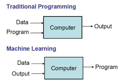
- Many useful programs learn something
- Basic Paradigm
- Observe set of examples: training data
- Infer something about process that generated that data
- Use inference to make predictions about previously unseen data: test data
- All ML Methods Require
- Representation of the features
- Distance metric for feature vectors
- Objective function and constraints
- Optimization method for learning the model
- Evaluation method
- Supervised Learning
- Start with set of feature vector / value pairs
- Goal : find a model that predicts a value for a previously unseen feature vector
-
Regression models predict a real
- E.g. linear regression
- Classification models predict a label (chosen from a finite set of labels)
- Unsupervied Learning
- Start with a set of feature vectors
- Goal : uncover some latent structure in the set of feature vectors
-
Clustering the most common technique
- Define some metric that captures how similar one feature vector is to another
- Group examples based on this metric
- Choosing Features
- Features never fully describe the situation
- Feature Engineering
- Represent examples by feature vectors that will facilitate generalization
- Suppose I want to use 100 examples from past to predict which students will pass the final exam
- Some features surely helpful, e.g., their grade on the midterm, did they do the problem sets, etc.
- Others might cause me to overfit, e.g., birth month
- Whant to maximize ratio of useful input to irrelevant input
- Signal-to-Noise Ratio (SNR)
- K-Nearest Neighbors
- Distance between vectors
- Minkowski metric $$ dist(X_1, X_2, p) = (\sum_{k=1}^{len}abs({X_1}_k - {X_2}_k)^p)^{\frac{1}{p}} \\ p=1 : \text{Manhattan Distance} \\ p=2 : \text{Euclidean Distance}$$
- Distance between vectors
from lecture12_segment2 import *
cobra = Animal('cobra', [1,1,1,1,0])
rattlesnake = Animal('rattlesnake', [1,1,1,1,0])
boa = Animal('boa\nconstrictor', [0,1,0,1,0])
chicken = Animal('chicken', [1,1,0,1,2])
alligator = Animal('alligator', [1,1,0,1,4])
dartFrog = Animal('dart frog', [1,0,1,0,4])
zebra = Animal('zebra', [0,0,0,0,4])
python = Animal('python', [1,1,0,1,0])
guppy = Animal('guppy', [0,1,0,0,0])
animals = [cobra, rattlesnake, boa, chicken, guppy,
           dartFrog, zebra, python, alligator]
compareAnimals(animals, 3) # k=3

- Using Distance Matrix for classification
- Simplest approach is probably nearest neighbor
- Remember training data
- When predicting the label of a new example
- Find the nearest example in the training data
- Predict the label associated with that example
- Advantage and Disadvantage of KNN
- Advantages
- Learning fase, no explicit training
- No theory required
- Easy to explain method and results
- Disadvantages
- Memory intensive and predictions can take a long time
- Are better algorithms than brute force
- No model to shed light on process that generated data
- Memory intensive and predictions can take a long time
- Advantages
cobra = Animal('cobra', [1,1,1,1,0])
rattlesnake = Animal('rattlesnake', [1,1,1,1,0])
boa = Animal('boa\nconstrictor', [0,1,0,1,0])
chicken = Animal('chicken', [1,1,0,1,2])
alligator = Animal('alligator', [1,1,0,1,1])
dartFrog = Animal('dart frog', [1,0,1,0,1])
zebra = Animal('zebra', [0,0,0,0,1])
python = Animal('python', [1,1,0,1,0])
guppy = Animal('guppy', [0,1,0,0,0])
animals = [cobra, rattlesnake, boa, chicken, guppy,
          dartFrog, zebra, python, alligator]
compareAnimals(animals, 3) k = 3

- A more General Approach: Scaling
- Z-scaling
- Each feature has a mean of 0 & a standard deviation of 1
- Interpolation
- Map minimum value to 0, maximum value to 1, and linearly interpolate ```python def zScaleFeatures(vals): """Assumes vals is a sequence of floats""" result = np.array(vals) mean = np.mean(vals) result = result - mean return result/np.std(result)
- Z-scaling
def iScaleFeatures(vals): """Assumes vals is a sequence of floats""" minVal, maxVal = min(vals), max(vals) fit = np.polyfit([minVal, maxVal], [0, 1], 1) return np.polyval(fit, vals) ```
- Clustering
- Partition examples into groups (clusters) such that examples in a group are more similar to each other than to examples in other groups
- Unlike classification, there is not typically a "right answer"
- Answer dictated by feature vector and distance metric, not by a group truth label
- Optimization Problem
$$ variability(c) = \sum_{e \in c} distance(mean(c), e)^2 \\
dissimilarity(C) = \sum_{c \in C} variability(c) \\
c :\text{one cluster} \\
C : \text{all of the clusters}$$
- Why not divide variability by size of cluster?
- Big and bad worse than small and bad
- Is optimization problem finding a $C$ that minimizes $dissimilarity(C)$?
- No, otherwise could put each example in its own cluster
- Need constraints, e.g.
- Minimum distance between clusters
- Number of clusters
- Why not divide variability by size of cluster?
- K-means Clustering
- Constraint: exactly k non-empty clusters
- Use a greedy algorithm to find an approximation to minimizing objective function
- Algorithm
randomly chose k examples as initial centroids
while true:
  create k clusters by assigning each example to closest centroid
  compute k new centroids by averaging examples in each cluster
  if centroids don`t change:
      break
from lecture12_segment3 import *
centers = [(2, 3), (4, 6), (7, 4), (7,7)]
examples = []
random.seed(0)
for c in centers:
    for i in range(5):
        xVal = (c[0] + random.gauss(0, .5))
        yVal = (c[1] + random.gauss(0, .5))
        name = str(c) + '-' + str(i)
        example = Example(name, pylab.array([xVal, yVal]))
        examples.append(example)

xVals, yVals = [], []
for e in examples:
    xVals.append(e.getFeatures()[0])
    yVals.append(e.getFeatures()[1])

random.seed(2)
kmeans(examples, 4, True)


- Mitigating Dependence on Initial Centroids
best = kMeans(points)
for t in range(numTrials):
  C = kMeans(points)
  if dissimilarity(C) < dissimilarity(best):
      best = C
return best
- A Pretty Example
- User k-means to cluster groups of pixels in an image by their color
- Get the color associated with the centroid of each cluster, i.e., the average color of the cluster
- For each pixel in the original image, find the centroid that is its nearest neighbor
- Replaced the pixel by that centroid